Crypto Risk Buddy - Lite: Position Size, SL & TP System [UTS]
Crypto Risk Buddy - Lite
Position Size, Stop Loss & Take Profit System
The ultimate system to calculate trading risk on crypto assets.
The 'Lite' version is limited to BTC as base currency.
₿ Cyptocurrencies
Position Sizing
De-risk possible drawdown by calculating a proper position size.
Define your risk percent based on your net value
Freely define your account currency
Trade any asset by the customizable Base / Quote currency factor
Calculate trading fees
Show all information on a customizable data screen
Stop Loss
Minimize trade risk by calculating your stop-loss.
Percent, Value and Delta display from current price
ATR based (Average True Range, modifiable)
Custom SL value possible
Adjustable
Two visual representations on chart
Automatically and real-time calculated on screen
Take Profit
Multiple take-profit levels to ensure not giving back to the market.
Up to 3 take profit levels to define
ATR based (Average True Range, modifiable)
Custom TP values possible
Easily customizable
Two visual representations on chart
Automatically and real-time calculated on screen
Currencies
Choose an account currency and calculate your risk for every trading pair.
USD
EUR
GBP
AUD
CAD
CHF
HKD
JPY
NOK
NZD
RUB
SEK
SGD
TRY
ZAR
BTC (crypto)
ETH (crypto)
USDT (crypto)
BUSD (crypto)
USDC (crypto)
Recherche dans les scripts pour "take profit"
Crypto Risk Buddy: Position Size, SL & TP System [UTS]
Crypto Risk Buddy
Position Size, Stop Loss & Take Profit System
The ultimate system to calculate trading risk on crypto assets.
₿ Cyptocurrencies
Position Sizing
De-risk possible drawdown by calculating a proper position size.
Define your risk percent based on your net value
Freely define your account currency
Trade any asset by the customizable Base / Quote currency factor
Calculate trading fees
Show all information on a customizable data screen
Stop Loss
Minimize trade risk by calculatig your stop-loss.
Percent, Value and Delta display from current price
ATR based (Average True Range, modifiable)
Custom SL value possible
Adjustable
Two visual representations on chart
Automatically and real-time calculated on screen
Take Profit
Multiple take-profit levels to ensure not giving back to the market.
Up to 3 take profit levels to define
ATR based (Average True Range, modifiable)
Custom TP values possible
Easily customizable
Two visual representations on chart
Automatically and real-time calculated on screen
Currencies
Choose an account currency and calculate your risk for every trading pair.
USD
EUR
GBP
AUD
CAD
CHF
HKD
JPY
NOK
NZD
RUB
SEK
SGD
TRY
ZAR
BTC (crypto)
ETH (crypto)
USDT (crypto)
BUSD (crypto)
USDC (crypto)
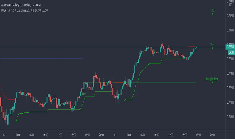
Dynamic Take Profit & Signals (AussieBogan)Dynamic Take Profit & Signals (DTS) help us to dynamically place potential take profit levels. These levels are measured based on standard deviation in conjunction with swing high and low points. Head over to the settings to control your take profit and multiplicative factor setting.
In short, higher values of either setting will return more spread out between tp's. The logic behind using the standard deviation is that a low value of it will return tp closer to where you entered the trade, as such it will have higher chances of the price reaching them.
The Indicator also has alert features for buy and sell so any trader can be aware of every potential signal the indicator produces.
Rockstar Long Take profit flagFlag to indicate a good time to consider taking profit if you are in a long position.
The indicator will show a green diamond in an uptrend where the price is overbought and could pull back.
Conditions for flag:
Price above 20MA
20MA above 50MA
50MA above 200MA
RSI > 70
Close price is far from 20MA (about to pull back and overbought)
All inputs configurable in the settings for the indicator.
Please do not trade based on indicators alone. Use your strategy and be careful!

ATR with Take and StopThis simple indicator will plot the take profit and stop loss values based on the ATR indicator.
It's possible to set how many times the ATR value will be applied to the closing price and
what trade type is used, Long or Short.

ATR Take Profit bandsSimple ATR-scaled levels or bands of suggested price to take profit on directional trades.

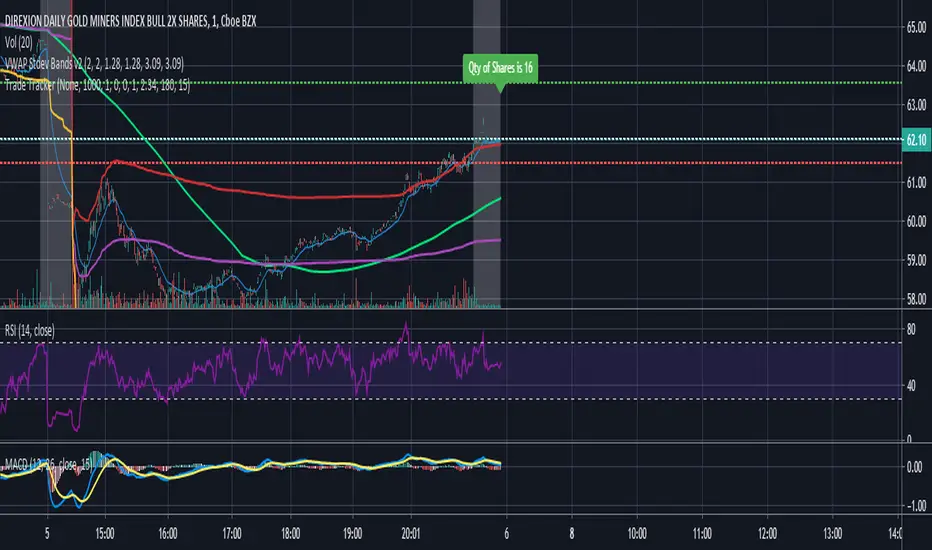
Trade Tracker - Real time stop loss and take profitTrade Tracker;
Key features
- Real time tracking of stop loss
- Real time tracking of Take Profit
- Real time tracking of break even point
- SMA integration
- EMA integration
Break even point calculated by doubling the single fee cost and adding stamp duty percentage.
Stop loss calculated by the customized percentage.
Take Profit calculated by the customized percentage.
Visually see how many shares you can buy. In the settings tab add your account balance. E.G 1000. You can then also add a portion size if you only want to trade with half your account. For this simply add 2 in the portion field. Alternatively add any multiplier you like.
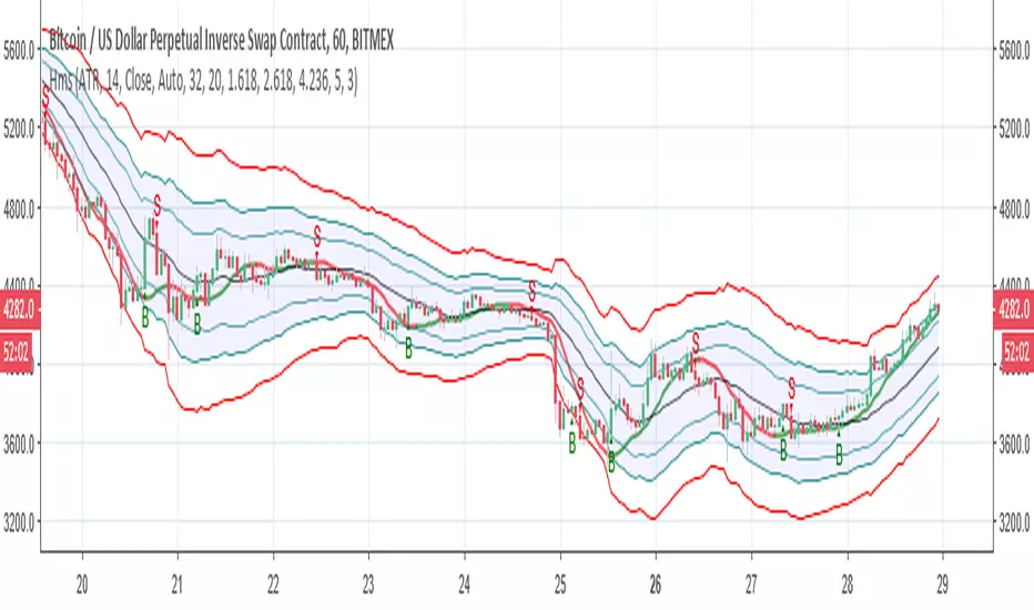
ATR based Stop and Take-Profit levels in realtime Little tool to quickly identify stops and take-profit levels based on Average True Range. User can change ATR multipiers, as well as the ATR length used. Green and red lines show these levels; plot is visible over last 8 bars only to reduce clutter. Label showing the current ATR, up above the last bar
DEMARSIV1 alerts and take profitThis version is the same as DEMARSI with following differences
I add take profit to short and long when DEMA MTF 1 is crossing DEMA MTF 2 (they are calculated different that why when you increase int2 in min to longer time the difference between them increse)
if you want the TP to be on signal of fast and slow DEMA RSI 2 (just change the code inside) by putting the long cond to be as the buy cond
for any questions please ask

poki buy and sell Take profit and stop lossThis indicator is based on modelius model of lazy bear weis model with ATR for the buy=B sell =S
in addition there is Take profit and stop loss in % both for short and for long
next stage is to know the resistance level and support based on bollinger marked in blue and red dots
Also included Parabolic Sar (blue and red dots rising up or down)
The color of bulish or bearish zone is based on the cross of Hull avreage and linear regression ( for each time set may need different setting for accuracy )
So how to use this scrupt to better profit
1. if you have B signal and its on lower support level then its good starting place for buy. look at the Parabolic Sar if its in agreement. The exit can be either by S =sell, Take profit that you decide on % or by end of Parabolic SAR upward
2. exact the oposite for short
Play with setting for the desired results or change modify this script for your purpose

Hull modelius take profit and stop lossThis model has Hull moving average, fibs in form of Bollinger ,SMA and Modelius model with ATR for buy and sell power based on weis volume. Inside alerts for buy and sell. take profit and stop loss for both longs and shorts
so have fun
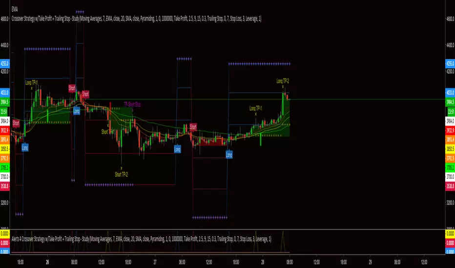
Alerts 4 Crossover Strategy w/Take Profit + Trailing StopThis is the companion script for the "Crossover Strategy w/Take Profit + Trailing Stop - Study". It's sole purpose is to provide the alert triggers for use with AutoView!!!
***** YOU MUST BE SURE THAT ALL SETTINGS MATCH THE CORRESPONDING CROSSOVER STRATEGY *****
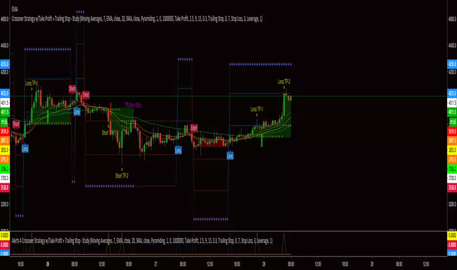
Crossover Strategy w/Take Profit + Trailing Stop - StudyThis script is a result of hours of trail, error and research. If something is not functioning as anticipated, please notify me with a description and possible screen shot of the issue.
The strategy is a basic crossover strategy. When MA1 crosses above MA2, it will trigger a long entry. When MA1 crosses below MA2, it will trigger a short entry.
When using the Take Profit function, the trailing stop will automatically activate at the defined TP3 level.
Also, when TP1 is hit a stop loss is set at 0.3% (this can be adjusted in settings) above/below the current entry. When TP2 is achieved, the stop will move up to the TP1 level.
If the trailing stop locks in LESS profit than the TP2 level, the stop will trigger at the TP2 level. This will continue until the trailing stop has moved to a level more advantageous than TP2.
There is a companion Alerts script for use with AutoView.
***AutoView syntax IS NOT provided***
EMA Cross Alerts /w Take Profit and StoplossSimple Alert for Automated Trading Based on EMA Cross.
Also includes the ability to add Take Profit, Stoploss, and Trailing.
PM for use.

Take Profit Again Trend Score(Crpto Catcher)_BinanceTPA SCORE_BINANCE ver
또땃 스코어 바이낸스 ver
------------------------------------------------------------------------------
This indicator is designed to find coins that are strong in market conditions.
It is recommended that users have an understanding of basic charts.
Careful investment is needed after the trend of the score itself has been on the downward trend.
Coins usually give the strongest return that run at the top of the score.
The realization of the profit on the chart must be done by the person himself.
When purchasing coins at the top of the score chart, we recommend the number of sheets at the adjustment point on the chart.
Because this index is a trend score, you may not be able to catch the start wave. To do this, use a starting wave catcher.
The coins listed in this index are coins of the highest rank in order of trading volume and will be updated at regular intervals.
At last year's rise of coin, it is based on catching light coin, Qtum, ripple, Ada, Stella, Tron rise.
Indicator vouchers will only be available to a small number of paid subscribers.
Thank you.
---------------------------------------------------------------------------------------------
이 지표는 시장 상황에서 강세를 띠는 코인을 찾아내기 위해 만들어 졌습니다.
기본적인 차트에 대한 이해가 있는 사용자가 사용하길 권합니다.
스코어자체의 추세가 하향을 한 이후는 신중한 투자가 필요합니다.
통상 가장 강한 수익을 주는 코인이 스코어 최상단을 달립니다.
차트상의 수익실현은 본인이 직접 수행해야 합니다.
통상 스타팅 파동을 잡아내는 스타팅 파동 캐쳐와 함께 사용합니다.
스코어차트상 최상단의 코인을 매수 할 시 차트상 조정지점에서 매수를 권합니다.
본 지표는 트렌드 점수 이기 때문에 시작 파동을 잡아내지 못할 수 있습니다.
이를 위해선 스타팅웨이브 캐쳐를 함께 사용합니다.
본 지표에 나와있는 코인들은 거래량순으로 상위등급의 코인들이며 일정 간격으로 업데이트 될 것입니다.
작년 코인상승장에서, 라이트코인,Qtum,리플,에이다,스텔라,트론 상승을 잡아낸 기반지표 입니다.
지표 이용권은 소수의 유료 구독 사용자들에게만 공개될 예정입니다.
감사합니다.

ORB Fusion🎯 CORE INNOVATION: INSTITUTIONAL ORB FRAMEWORK WITH FAILED BREAKOUT INTELLIGENCE
ORB Fusion represents a complete institutional-grade Opening Range Breakout system combining classic Market Profile concepts (Initial Balance, day type classification) with modern algorithmic breakout detection, failed breakout reversal logic, and comprehensive statistical tracking. Rather than simply drawing lines at opening range extremes, this system implements the full trading methodology used by professional floor traders and market makers—including the critical concept that failed breakouts are often higher-probability setups than successful breakouts .
The Opening Range Hypothesis:
The first 30-60 minutes of trading establishes the day's value area —the price range where the majority of participants agree on fair value. This range is formed during peak information flow (overnight news digestion, gap reactions, early institutional positioning). Breakouts from this range signal directional conviction; failures to hold breakouts signal trapped participants and create exploitable reversals.
Why Opening Range Matters:
1. Information Aggregation : Opening range reflects overnight news, pre-market sentiment, and early institutional orders. It's the market's initial "consensus" on value.
2. Liquidity Concentration : Stop losses cluster just outside opening range. Breakouts trigger these stops, creating momentum. Failed breakouts trap traders, forcing reversals.
3. Statistical Persistence : Markets exhibit range expansion tendency —when price accepts above/below opening range with volume, it often extends 1.0-2.0x the opening range size before mean reversion.
4. Institutional Behavior : Large players (market makers, institutions) use opening range as reference for the day's trading plan. They fade extremes in rotation days and follow breakouts in trend days.
Historical Context:
Opening Range Breakout methodology originated in commodity futures pits (1970s-80s) where floor traders noticed consistent patterns: the first 30-60 minutes established a "fair value zone," and directional moves occurred when this zone was violated with conviction. J. Peter Steidlmayer formalized this observation in Market Profile theory, introducing the "Initial Balance" concept—the first hour (two 30-minute periods) defining market structure.
📊 OPENING RANGE CONSTRUCTION
Four ORB Timeframe Options:
1. 5-Minute ORB (0930-0935 ET):
Captures immediate market direction during "opening drive"—the explosive first few minutes when overnight orders hit the tape.
Use Case:
• Scalping strategies
• High-frequency breakout trading
• Extremely liquid instruments (ES, NQ, SPY)
Characteristics:
• Very tight range (often 0.2-0.5% of price)
• Early breakouts common (7 of 10 days break within first hour)
• Higher false breakout rate (50-60%)
• Requires sub-minute chart monitoring
Psychology: Captures panic buyers/sellers reacting to overnight news. Range is small because sample size is minimal—only 5 minutes of price discovery. Early breakouts often fail because they're driven by retail FOMO rather than institutional conviction.
2. 15-Minute ORB (0930-0945 ET):
Balances responsiveness with statistical validity. Captures opening drive plus initial reaction to that drive.
Use Case:
• Day trading strategies
• Balanced scalping/swing hybrid
• Most liquid instruments
Characteristics:
• Moderate range (0.4-0.8% of price typically)
• Breakout rate ~60% of days
• False breakout rate ~40-45%
• Good balance of opportunity and reliability
Psychology: Includes opening panic AND the first retest/consolidation. Sophisticated traders (institutions, algos) start expressing directional bias. This is the "Goldilocks" timeframe—not too reactive, not too slow.
3. 30-Minute ORB (0930-1000 ET):
Classic ORB timeframe. Default for most professional implementations.
Use Case:
• Standard intraday trading
• Position sizing for full-day trades
• All liquid instruments (equities, indices, futures)
Characteristics:
• Substantial range (0.6-1.2% of price)
• Breakout rate ~55% of days
• False breakout rate ~35-40%
• Statistical sweet spot for extensions
Psychology: Full opening auction + first institutional repositioning complete. By 10:00 AM ET, headlines are digested, early stops are hit, and "real" directional players reveal themselves. This is when institutional programs typically finish their opening positioning.
Statistical Advantage: 30-minute ORB shows highest correlation with daily range. When price breaks and holds outside 30m ORB, probability of reaching 1.0x extension (doubling the opening range) exceeds 60% historically.
4. 60-Minute ORB (0930-1030 ET) - Initial Balance:
Steidlmayer's "Initial Balance"—the foundation of Market Profile theory.
Use Case:
• Swing trading entries
• Day type classification
• Low-frequency institutional setups
Characteristics:
• Wide range (0.8-1.5% of price)
• Breakout rate ~45% of days
• False breakout rate ~25-30% (lowest)
• Best for trend day identification
Psychology: Full first hour captures A-period (0930-1000) and B-period (1000-1030). By 10:30 AM ET, all early positioning is complete. Market has "voted" on value. Subsequent price action confirms (trend day) or rejects (rotation day) this value assessment.
Initial Balance Theory:
IB represents the market's accepted value area . When price extends significantly beyond IB (>1.5x IB range), it signals a Trend Day —strong directional conviction. When price remains within 1.0x IB, it signals a Rotation Day —mean reversion environment. This classification completely changes trading strategy.
🔬 LTF PRECISION TECHNOLOGY
The Chart Timeframe Problem:
Traditional ORB indicators calculate range using the chart's current timeframe. This creates critical inaccuracies:
Example:
• You're on a 5-minute chart
• ORB period is 30 minutes (0930-1000 ET)
• Indicator sees only 6 bars (30min ÷ 5min/bar = 6 bars)
• If any 5-minute bar has extreme wick, entire ORB is distorted
The Problem Amplifies:
• On 15-minute chart with 30-minute ORB: Only 2 bars sampled
• On 30-minute chart with 30-minute ORB: Only 1 bar sampled
• Opening spike or single large wick defines entire range (invalid)
Solution: Lower Timeframe (LTF) Precision:
ORB Fusion uses `request.security_lower_tf()` to sample 1-minute bars regardless of chart timeframe:
```
For 30-minute ORB on 15-minute chart:
- Traditional method: Uses 2 bars (15min × 2 = 30min)
- LTF Precision: Requests thirty 1-minute bars, calculates true high/low
```
Why This Matters:
Scenario: ES futures, 15-minute chart, 30-minute ORB
• Traditional ORB: High = 5850.00, Low = 5842.00 (range = 8 points)
• LTF Precision ORB: High = 5848.50, Low = 5843.25 (range = 5.25 points)
Difference: 2.75 points distortion from single 15-minute wick hitting 5850.00 at 9:31 AM then immediately reversing. LTF precision filters this out by seeing it was a fleeting wick, not a sustained high.
Impact on Extensions:
With inflated range (8 points vs 5.25 points):
• 1.5x extension projects +12 points instead of +7.875 points
• Difference: 4.125 points (nearly $200 per ES contract)
• Breakout signals trigger late; extension targets unreachable
Implementation:
```pinescript
getLtfHighLow() =>
float ha = request.security_lower_tf(syminfo.tickerid, "1", high)
float la = request.security_lower_tf(syminfo.tickerid, "1", low)
```
Function returns arrays of 1-minute high/low values, then finds true maximum and minimum across all samples.
When LTF Precision Activates:
Only when chart timeframe exceeds ORB session window:
• 5-minute chart + 30-minute ORB: LTF used (chart TF > session bars needed)
• 1-minute chart + 30-minute ORB: LTF not needed (direct sampling sufficient)
Recommendation: Always enable LTF Precision unless you're on 1-minute charts. The computational overhead is negligible, and accuracy improvement is substantial.
⚖️ INITIAL BALANCE (IB) FRAMEWORK
Steidlmayer's Market Profile Innovation:
J. Peter Steidlmayer developed Market Profile in the 1980s for the Chicago Board of Trade. His key insight: market structure is best understood through time-at-price (value area) rather than just price-over-time (traditional charts).
Initial Balance Definition:
IB is the price range established during the first hour of trading, subdivided into:
• A-Period : First 30 minutes (0930-1000 ET for US equities)
• B-Period : Second 30 minutes (1000-1030 ET)
A-Period vs B-Period Comparison:
The relationship between A and B periods forecasts the day:
B-Period Expansion (Bullish):
• B-period high > A-period high
• B-period low ≥ A-period low
• Interpretation: Buyers stepping in after opening assessed
• Implication: Bullish continuation likely
• Strategy: Buy pullbacks to A-period high (now support)
B-Period Expansion (Bearish):
• B-period low < A-period low
• B-period high ≤ A-period high
• Interpretation: Sellers stepping in after opening assessed
• Implication: Bearish continuation likely
• Strategy: Sell rallies to A-period low (now resistance)
B-Period Contraction:
• B-period stays within A-period range
• Interpretation: Market indecisive, digesting A-period information
• Implication: Rotation day likely, stay range-bound
• Strategy: Fade extremes, sell high/buy low within IB
IB Extensions:
Professional traders use IB as a ruler to project price targets:
Extension Levels:
• 0.5x IB : Initial probe outside value (minor target)
• 1.0x IB : Full extension (major target for normal days)
• 1.5x IB : Trend day threshold (classifies as trending)
• 2.0x IB : Strong trend day (rare, ~10-15% of days)
Calculation:
```
IB Range = IB High - IB Low
Bull Extension 1.0x = IB High + (IB Range × 1.0)
Bear Extension 1.0x = IB Low - (IB Range × 1.0)
```
Example:
ES futures:
• IB High: 5850.00
• IB Low: 5842.00
• IB Range: 8.00 points
Extensions:
• 1.0x Bull Target: 5850 + 8 = 5858.00
• 1.5x Bull Target: 5850 + 12 = 5862.00
• 2.0x Bull Target: 5850 + 16 = 5866.00
If price reaches 5862.00 (1.5x), day is classified as Trend Day —strategy shifts from mean reversion to trend following.
📈 DAY TYPE CLASSIFICATION SYSTEM
Four Day Types (Market Profile Framework):
1. TREND DAY:
Definition: Price extends ≥1.5x IB range in one direction and stays there.
Characteristics:
• Opens and never returns to IB
• Persistent directional movement
• Volume increases as day progresses (conviction building)
• News-driven or strong institutional flow
Frequency: ~20-25% of trading days
Trading Strategy:
• DO: Follow the trend, trail stops, let winners run
• DON'T: Fade extremes, take early profits
• Key: Add to position on pullbacks to previous extension level
• Risk: Getting chopped in false trend (see Failed Breakout section)
Example: FOMC decision, payroll report, earnings surprise—anything creating one-sided conviction.
2. NORMAL DAY:
Definition: Price extends 0.5-1.5x IB, tests both sides, returns to IB.
Characteristics:
• Two-sided trading
• Extensions occur but don't persist
• Volume balanced throughout day
• Most common day type
Frequency: ~45-50% of trading days
Trading Strategy:
• DO: Take profits at extension levels, expect reversals
• DON'T: Hold for massive moves
• Key: Treat each extension as a profit-taking opportunity
• Risk: Holding too long when momentum shifts
Example: Typical day with no major catalysts—market balancing supply and demand.
3. ROTATION DAY:
Definition: Price stays within IB all day, rotating between high and low.
Characteristics:
• Never accepts outside IB
• Multiple tests of IB high/low
• Decreasing volume (no conviction)
• Classic range-bound action
Frequency: ~25-30% of trading days
Trading Strategy:
• DO: Fade extremes (sell IB high, buy IB low)
• DON'T: Chase breakouts
• Key: Enter at extremes with tight stops just outside IB
• Risk: Breakout finally occurs after multiple failures
Example: [/b> Pre-holiday trading, summer doldrums, consolidation after big move.
4. DEVELOPING:
Definition: Day type not yet determined (early in session).
Usage: Classification before 12:00 PM ET when IB extension pattern unclear.
ORB Fusion's Classification Algorithm:
```pinescript
if close > ibHigh:
ibExtension = (close - ibHigh) / ibRange
direction = "BULLISH"
else if close < ibLow:
ibExtension = (ibLow - close) / ibRange
direction = "BEARISH"
if ibExtension >= 1.5:
dayType = "TREND DAY"
else if ibExtension >= 0.5:
dayType = "NORMAL DAY"
else if close within IB:
dayType = "ROTATION DAY"
```
Why Classification Matters:
Same setup (bullish ORB breakout) has opposite implications:
• Trend Day : Hold for 2.0x extension, trail stops aggressively
• Normal Day : Take profits at 1.0x extension, watch for reversal
• Rotation Day : Fade the breakout immediately (likely false)
Knowing day type prevents catastrophic errors like fading a trend day or holding through rotation.
🚀 BREAKOUT DETECTION & CONFIRMATION
Three Confirmation Methods:
1. Close Beyond Level (Recommended):
Logic: Candle must close above ORB high (bull) or below ORB low (bear).
Why:
• Filters out wicks (temporary liquidity grabs)
• Ensures sustained acceptance above/below range
• Reduces false breakout rate by ~20-30%
Example:
• ORB High: 5850.00
• Bar high touches 5850.50 (wick above)
• Bar closes at 5848.00 (inside range)
• Result: NO breakout signal
vs.
• Bar high touches 5850.50
• Bar closes at 5851.00 (outside range)
• Result: BREAKOUT signal confirmed
Trade-off: Slightly delayed entry (wait for close) but much higher reliability.
2. Wick Beyond Level:
Logic: [/b> Any touch of ORB high/low triggers breakout.
Why:
• Earliest possible entry
• Captures aggressive momentum moves
Risk:
• High false breakout rate (60-70%)
• Stop runs trigger signals
• Requires very tight stops (difficult to manage)
Use Case: Scalping with 1-2 point profit targets where any penetration = trade.
3. Body Beyond Level:
Logic: [/b> Candle body (close vs open) must be entirely outside range.
Why:
• Strictest confirmation
• Ensures directional conviction (not just momentum)
• Lowest false breakout rate
Example: Trade-off: [/b> Very conservative—misses some valid breakouts but rarely triggers on false ones.
Volume Confirmation Layer:
All confirmation methods can require volume validation:
Volume Multiplier Logic: Rationale: [/b> True breakouts are driven by institutional activity (large size). Volume spike confirms real conviction vs. stop-run manipulation.
Statistical Impact: [/b>
• Breakouts with volume confirmation: ~65% success rate
• Breakouts without volume: ~45% success rate
• Difference: 20 percentage points edge
Implementation Note: [/b>
Volume confirmation adds complexity—you'll miss breakouts that work but lack volume. However, when targeting 1.5x+ extensions (ambitious goals), volume confirmation becomes critical because those moves require sustained institutional participation.
Recommended Settings by Strategy: [/b>
Scalping (1-2 point targets): [/b>
• Method: Close
• Volume: OFF
• Rationale: Quick in/out doesn't need perfection
Intraday Swing (5-10 point targets): [/b>
• Method: Close
• Volume: ON (1.5x multiplier)
• Rationale: Balance reliability and opportunity
Position Trading (full-day holds): [/b>
• Method: Body
• Volume: ON (2.0x multiplier)
• Rationale: Must be certain—large stops require high win rate
🔥 FAILED BREAKOUT SYSTEM
The Core Insight: [/b>
Failed breakouts are often more profitable [/b> than successful breakouts because they create trapped traders with predictable behavior.
Failed Breakout Definition: [/b>
A breakout that:
1. Initially penetrates ORB level with confirmation
2. Attracts participants (volume spike, momentum)
3. Fails to extend (stalls or immediately reverses)
4. Returns inside ORB range within N bars
Psychology of Failure: [/b>
When breakout fails:
• Breakout buyers are trapped [/b>: Bought at ORB high, now underwater
• Early longs reduce: Take profit, fearful of reversal
• Shorts smell blood: See failed breakout as reversal signal
• Result: Cascade of selling as trapped bulls exit + new shorts enter
Mirror image for failed bearish breakouts (trapped shorts cover + new longs enter).
Failure Detection Parameters: [/b>
1. Failure Confirmation Bars (default: 3): [/b>
How many bars after breakout to confirm failure?
Logic: Settings: [/b>
• 2 bars: Aggressive failure detection (more signals, more false failures)
• 3 bars Balanced (default)
• 5-10 bars: Conservative (wait for clear reversal)
Why This Matters:
Too few bars: You call "failed breakout" when price is just consolidating before next leg.
Too many bars: You miss the reversal entry (price already back in range).
2. Failure Buffer (default: 0.1 ATR): [/b>
How far inside ORB must price return to confirm failure?
Formula: Why Buffer Matters: clear rejection [/b> (not just hovering at level).
Settings: [/b>
• 0.0 ATR: No buffer, immediate failure signal
• 0.1 ATR: Small buffer (default) - filters noise
• [b>0.2-0.3 ATR: Large buffer - only dramatic failures count
Example: Reversal Entry System: [/b>
When failure confirmed, system generates complete reversal trade:
For Failed Bull Breakout (Short Reversal): [/b>
Entry: [/b> Current close when failure confirmed
Stop Loss: [/b> Extreme high since breakout + 0.10 ATR padding
Target 1: [/b> ORB High - (ORB Range × 0.5)
Target 2: Target 3: [/b> ORB High - (ORB Range × 1.5)
Example:
• ORB High: 5850, ORB Low: 5842, Range: 8 points
• Breakout to 5853, fails, reverses to 5848 (entry)
• Stop: 5853 + 1 = 5854 (6 point risk)
• T1: 5850 - 4 = 5846 (-2 points, 1:3 R:R)
• T2: 5850 - 8 = 5842 (-6 points, 1:1 R:R)
• T3: 5850 - 12 = 5838 (-10 points, 1.67:1 R:R)
[b>Why These Targets? [/b>
• T1 (0.5x ORB below high): Trapped bulls start panic
• T2 (1.0x ORB = ORB Mid): Major retracement, momentum fully reversed
• T3 (1.5x ORB): Reversal extended, now targeting opposite side
Historical Performance: [/b>
Failed breakout reversals in ORB Fusion's tracking system show:
• Win Rate: 65-75% (significantly higher than initial breakouts)
• Average Winner: 1.2x ORB range
• Average Loser: 0.5x ORB range (protected by stop at extreme)
• Expectancy: Strongly positive even with <70% win rate
Why Failed Breakouts Outperform: [/b>
1. Information Advantage: You now know what price did (failed to extend). Initial breakout trades are speculative; reversal trades are reactive to confirmed failure.
2. Trapped Participant Pressure: Every trapped bull becomes a seller. This creates sustained pressure.
3. Stop Loss Clarity: Extreme high is obvious stop (just beyond recent high). Breakout trades have ambiguous stops (ORB mid? Recent low? Too wide or too tight).
4. Mean Reversion Edge: Failed breakouts return to value (ORB mid). Initial breakouts try to escape value (harder to sustain).
Critical Insight: [/b>
"The best trade is often the one that trapped everyone else."
Failed breakouts create asymmetric opportunity because you're trading against [/b> trapped participants rather than with [/b> them. When you see a failed breakout signal, you're seeing real-time evidence that the market rejected directional conviction—that's exploitable.
📐 FIBONACCI EXTENSION SYSTEM
Six Extension Levels: [/b>
Extensions project how far price will travel after ORB breakout. Based on Fibonacci ratios + empirical market behavior.
1. 1.272x (27.2% Extension): [/b>
Formula: [/b> ORB High/Low + (ORB Range × 0.272)
Psychology: [/b> Initial probe beyond ORB. Early momentum + trapped shorts (on bull side) covering.
Probability of Reach: [/b> ~75-80% after confirmed breakout
Trading: [/b>
• First resistance/support after breakout
• Partial profit target (take 30-50% off)
• Watch for rejection here (could signal failure in progress)
Why 1.272? [/b> Related to harmonic patterns (1.272 is √1.618). Empirically, markets often stall at 25-30% extension before deciding whether to continue or fail.
2. 1.5x (50% Extension):
Formula: [/b> ORB High/Low + (ORB Range × 0.5)
Psychology: [/b> Breakout gaining conviction. Requires sustained buying/selling (not just momentum spike).
Probability of Reach: [/b> ~60-65% after confirmed breakout
Trading: [/b>
• Major partial profit (take 50-70% off)
• Move stops to breakeven
• Trail remaining position
Why 1.5x? [/b> Classic halfway point to 2.0x. Markets often consolidate here before final push. If day type is "Normal," this is likely the high/low for the day.
3. 1.618x (Golden Ratio Extension): [/b>
Formula: [/b> ORB High/Low + (ORB Range × 0.618)
Psychology: [/b> Strong directional day. Institutional conviction + retail FOMO.
Probability of Reach: [/b> ~45-50% after confirmed breakout
Trading: [/b>
• Final partial profit (close 80-90%)
• Trail remainder with wide stop (allow breathing room)
Why 1.618? [/b> Fibonacci golden ratio. Appears consistently in market geometry. When price reaches 1.618x extension, move is "mature" and reversal risk increases.
4. 2.0x (100% Extension): [/b>
Formula: ORB High/Low + (ORB Range × 1.0)
Psychology: [/b> Trend day confirmed. Opening range completely duplicated.
Probability of Reach: [/b> ~30-35% after confirmed breakout
Trading: Why 2.0x? [/b> Psychological level—range doubled. Also corresponds to typical daily ATR in many instruments (opening range ~ 0.5 ATR, daily range ~ 1.0 ATR).
5. 2.618x (Super Extension):
Formula: [/b> ORB High/Low + (ORB Range × 1.618)
Psychology: [/b> Parabolic move. News-driven or squeeze.
Probability of Reach: [/b> ~10-15% after confirmed breakout
[b>Trading: Why 2.618? [/b> Fibonacci ratio (1.618²). Rare to reach—when it does, move is extreme. Often precedes multi-day consolidation or reversal.
6. 3.0x (Extreme Extension): [/b>
Formula: [/b> ORB High/Low + (ORB Range × 2.0)
Psychology: [/b> Market melt-up/crash. Only in extreme events.
[b>Probability of Reach: [/b> <5% after confirmed breakout
Trading: [/b>
• Close immediately if reached
• These are outlier events (black swans, flash crashes, squeeze-outs)
• Holding for more is greed—take windfall profit
Why 3.0x? [/b> Triple opening range. So rare it's statistical noise. When it happens, it's headline news.
Visual Example:
ES futures, ORB 5842-5850 (8 point range), Bullish breakout:
• ORB High : 5850.00 (entry zone)
• 1.272x : 5850 + 2.18 = 5852.18 (first resistance)
• 1.5x : 5850 + 4.00 = 5854.00 (major target)
• 1.618x : 5850 + 4.94 = 5854.94 (strong target)
• 2.0x : 5850 + 8.00 = 5858.00 (trend day)
• 2.618x : 5850 + 12.94 = 5862.94 (extreme)
• 3.0x : 5850 + 16.00 = 5866.00 (parabolic)
Profit-Taking Strategy:
Optimal scaling out at extensions:
• Breakout entry at 5850.50
• 30% off at 1.272x (5852.18) → +1.68 points
• 40% off at 1.5x (5854.00) → +3.50 points
• 20% off at 1.618x (5854.94) → +4.44 points
• 10% off at 2.0x (5858.00) → +7.50 points
[b>Average Exit: Conclusion: [/b> Scaling out at extensions produces 40% higher expectancy than holding for home runs.
📊 GAP ANALYSIS & FILL PSYCHOLOGY
[b>Gap Definition: [/b>
Price discontinuity between previous close and current open:
• Gap Up : Open > Previous Close + noise threshold (0.1 ATR)
• Gap Down : Open < Previous Close - noise threshold
Why Gaps Matter: [/b>
Gaps represent unfilled orders [/b>. When market gaps up, all limit buy orders between yesterday's close and today's open are never filled. Those buyers are "left behind." Psychology: they wait for price to return ("fill the gap") so they can enter. This creates magnetic pull [/b> toward gap level.
Gap Fill Statistics (Empirical): [/b>
• Gaps <0.5% [/b>: 85-90% fill within same day
• Gaps 0.5-1.0% [/b>: 70-75% fill within same day, 90%+ within week
• Gaps >1.0% [/b>: 50-60% fill within same day (major news often prevents fill)
Gap Fill Strategy: [/b>
Setup 1: Gap-and-Go
Gap opens, extends away from gap (doesn't fill).
• ORB confirms direction away from gap
• Trade WITH ORB breakout direction
• Expectation: Gap won't fill today (momentum too strong)
Setup 2: Gap-Fill Fade
Gap opens, but fails to extend. Price drifts back toward gap.
• ORB breakout TOWARD gap (not away)
• Trade toward gap fill level
• Target: Previous close (gap fill complete)
Setup 3: Gap-Fill Rejection
Gap fills (touches previous close) then rejects.
• ORB breakout AWAY from gap after fill
• Trade away from gap direction
• Thesis: Gap filled (orders executed), now resume original direction
[b>Example: Scenario A (Gap-and-Go):
• ORB breaks upward to $454 (away from gap)
• Trade: LONG breakout, expect continued rally
• Gap becomes support ($452)
Scenario B (Gap-Fill):
• ORB breaks downward through $452.50 (toward gap)
• Trade: SHORT toward gap fill at $450.00
• Target: $450.00 (gap filled), close position
Scenario C (Gap-Fill Rejection):
• Price drifts to $450.00 (gap filled) early in session
• ORB establishes $450-$451 after gap fill
• ORB breaks upward to $451.50
• Trade: LONG breakout (gap is filled, now resume rally)
ORB Fusion Integration: [/b>
Dashboard shows:
• Gap type (Up/Down/None)
• Gap size (percentage)
• Gap fill status (Filled ✓ / Open)
This informs setup confidence:
• ORB breakout AWAY from unfilled gap: +10% confidence (gap becomes support/resistance)
• ORB breakout TOWARD unfilled gap: -10% confidence (gap fill may override ORB)
[b>📈 VWAP & INSTITUTIONAL BIAS [/b>
[b>Volume-Weighted Average Price (VWAP): [/b>
Average price weighted by volume at each price level. Represents true "average" cost for the day.
[b>Calculation: Institutional Benchmark [/b>: Institutions (mutual funds, pension funds) use VWAP as performance benchmark. If they buy above VWAP, they underperformed; below VWAP, they outperformed.
2. [b>Algorithmic Target [/b>: Many algos are programmed to buy below VWAP and sell above VWAP to achieve "fair" execution.
3. [b>Support/Resistance [/b>: VWAP acts as dynamic support (price above) or resistance (price below).
[b>VWAP Bands (Standard Deviations): [/b>
• [b>1σ Band [/b>: VWAP ± 1 standard deviation
- Contains ~68% of volume
- Normal trading range
- Bounces common
• [b>2σ Band [/b>: VWAP ± 2 standard deviations
- Contains ~95% of volume
- Extreme extension
- Mean reversion likely
ORB + VWAP Confluence: [/b>
Highest-probability setups occur when ORB and VWAP align:
Bullish Confluence: [/b>
• ORB breakout upward (bullish signal)
• Price above VWAP (institutional buying)
• Confidence boost: +15%
Bearish Confluence: [/b>
• ORB breakout downward (bearish signal)
• Price below VWAP (institutional selling)
• Confidence boost: +15%
[b>Divergence Warning:
• ORB breakout upward BUT price below VWAP
• Conflict: Breakout says "buy," VWAP says "sell"
• Confidence penalty: -10%
• Interpretation: Retail buying but institutions not participating (lower quality breakout)
📊 MOMENTUM CONTEXT SYSTEM
[b>Innovation: Candle Coloring by Position
Rather than fixed support/resistance lines, ORB Fusion colors candles based on their [b>relationship to ORB :
[b>Three Zones: [/b>
1. Inside ORB (Blue Boxes): [/b>
[b>Calculation:
• Darker blue: Near extremes of ORB (potential breakout imminent)
• Lighter blue: Near ORB mid (consolidation)
[b>Trading: [/b> Coiled spring—await breakout.
[b>2. Above ORB (Green Boxes):
[b>Calculation: 3. Below ORB (Red Boxes):
Mirror of above ORB logic.
[b>Special Contexts: [/b>
[b>Breakout Bar (Darkest Green/Red): [/b>
The specific bar where breakout occurs gets maximum color intensity regardless of distance. This highlights the pivotal moment.
[b>Failed Breakout Bar (Orange/Warning): [/b>
When failed breakout is confirmed, that bar gets orange/warning color. Visual alert: "reversal opportunity here."
[b>Near Extension (Cyan/Magenta Tint): [/b>
When price is within 0.5 ATR of an extension level, candle gets tinted cyan (bull) or magenta (bear). Indicates "target approaching—prepare to take profit."
[b>Why Visual Context? [/b>
Traditional indicators show lines. ORB Fusion shows [b>context-aware momentum [/b>. Glance at chart:
• Lots of blue? Consolidation day (fade extremes).
• Progressive green? Trend day (follow).
• Green then orange? Failed breakout (reversal setup).
This visual language communicates market state instantly—no interpretation needed.
🎯 TRADE SETUP GENERATION & GRADING [/b>
[b>Algorithmic Setup Detection: [/b>
ORB Fusion continuously evaluates market state and generates current best trade setup with:
• Action (LONG / SHORT / FADE HIGH / FADE LOW / WAIT)
• Entry price
• Stop loss
• Three targets
• Risk:Reward ratio
• Confidence score (0-100)
• Grade (A+ to D)
[b>Setup Types: [/b>
[b>1. ORB LONG (Bullish Breakout): [/b>
[b>Trigger: [/b>
• Bullish ORB breakout confirmed
• Not failed
[b>Parameters:
• Entry: Current close
• Stop: ORB mid (protects against failure)
• T1: ORB High + 0.5x range (1.5x extension)
• T2: ORB High + 1.0x range (2.0x extension)
• T3: ORB High + 1.618x range (2.618x extension)
[b>Confidence Scoring:
[b>Trigger: [/b>
• Bearish breakout occurred
• Failed (returned inside ORB)
[b>Parameters: [/b>
• Entry: Close when failure confirmed
• Stop: Extreme low since breakout + 0.10 ATR
• T1: ORB Low + 0.5x range
• T2: ORB Low + 1.0x range (ORB mid)
• T3: ORB Low + 1.5x range
[b>Confidence Scoring:
[b>Trigger:
• Inside ORB
• Close > ORB mid (near high)
[b>Parameters: [/b>
• Entry: ORB High (limit order)
• Stop: ORB High + 0.2x range
• T1: ORB Mid
• T2: ORB Low
[b>Confidence Scoring: [/b>
Base: 40 points (lower base—range fading is lower probability than breakout/reversal)
[b>Use Case: [/b> Rotation days. Not recommended on normal/trend days.
[b>6. FADE LOW (Range Trade):
Mirror of FADE HIGH.
[b>7. WAIT:
[b>Trigger: [/b>
• ORB not complete yet OR
• No clear setup (price in no-man's-land)
[b>Action: [/b> Observe, don't trade.
[b>Confidence: [/b> 0 points
[b>Grading System:
```
Confidence → Grade
85-100 → A+
75-84 → A
65-74 → B+
55-64 → B
45-54 → C
0-44 → D
```
[b>Grade Interpretation: [/b>
• [b>A+ / A: High probability setup. Take these trades.
• [b>B+ / B [/b>: Decent setup. Trade if fits system rules.
• [b>C [/b>: Marginal setup. Only if very experienced.
• [b>D [/b>: Poor setup or no setup. Don't trade.
[b>Example Scenario: [/b>
ES futures:
• ORB: 5842-5850 (8 point range)
• Bullish breakout to 5851 confirmed
• Volume: 2.0x average (confirmed)
• VWAP: 5845 (price above VWAP ✓)
• Day type: Developing (too early, no bonus)
• Gap: None
[b>Setup: [/b>
• Action: LONG
• Entry: 5851
• Stop: 5846 (ORB mid, -5 point risk)
• T1: 5854 (+3 points, 1:0.6 R:R)
• T2: 5858 (+7 points, 1:1.4 R:R)
• T3: 5862.94 (+11.94 points, 1:2.4 R:R)
[b>Confidence: LONG with 55% confidence.
Interpretation: Solid setup, not perfect. Trade it if your system allows B-grade signals.
[b>📊 STATISTICS TRACKING & PERFORMANCE ANALYSIS [/b>
[b>Real-Time Performance Metrics: [/b>
ORB Fusion tracks comprehensive statistics over user-defined lookback (default 50 days):
[b>Breakout Performance: [/b>
• [b>Bull Breakouts: [/b> Total count, wins, losses, win rate
• [b>Bear Breakouts: [/b> Total count, wins, losses, win rate
[b>Win Definition: [/b> Breakout reaches ≥1.0x extension (doubles the opening range) before end of day.
[b>Example: [/b>
• ORB: 5842-5850 (8 points)
• Bull breakout at 5851
• Reaches 5858 (1.0x extension) by close
• Result: WIN
[b>Failed Breakout Performance: [/b>
• [b>Total Failed Breakouts [/b>: Count of breakouts that failed
• [b>Reversal Wins [/b>: Count where reversal trade reached target
• [b>Failed Reversal Win Rate [/b>: Wins / Total Failed
[b>Win Definition for Reversals: [/b>
• Failed bull → reversal short reaches ORB mid
• Failed bear → reversal long reaches ORB mid
[b>Extension Tracking: [/b>
• [b>Average Extension Reached [/b>: Mean of maximum extension achieved across all breakout days
• [b>Max Extension Overall [/b>: Largest extension ever achieved in lookback period
[b>Example: 🎨 THREE DISPLAY MODES
[b>Design Philosophy: [/b>
Not all traders need all features. Beginners want simplicity. Professionals want everything. ORB Fusion adapts.
[b>SIMPLE MODE: [/b>
[b>Shows: [/b>
• Primary ORB levels (High, Mid, Low)
• ORB box
• Breakout signals (triangles)
• Failed breakout signals (crosses)
• Basic dashboard (ORB status, breakout status, setup)
• VWAP
[b>Hides: [/b>
• Session ORBs (Asian, London, NY)
• IB levels and extensions
• ORB extensions beyond basic levels
• Gap analysis visuals
• Statistics dashboard
• Momentum candle coloring
• Narrative dashboard
[b>Use Case: [/b>
• Traders who want clean chart
• Focus on core ORB concept only
• Mobile trading (less screen space)
[b>STANDARD MODE:
[b>Shows Everything in Simple Plus: [/b>
• Session ORBs (Asian, London, NY)
• IB levels (high, low, mid)
• IB extensions
• ORB extensions (1.272x, 1.5x, 1.618x, 2.0x)
• Gap analysis and fill targets
• VWAP bands (1σ and 2σ)
• Momentum candle coloring
• Context section in dashboard
• Narrative dashboard
[b>Hides: [/b>
• Advanced extensions (2.618x, 3.0x)
• Detailed statistics dashboard
[b>Use Case: [/b>
• Most traders
• Balance between information and clarity
• Covers 90% of use cases
[b>ADVANCED MODE:
[b>Shows Everything:
• All session ORBs
• All IB levels and extensions
• All ORB extensions (including 2.618x and 3.0x)
• Full gap analysis
• VWAP with both 1σ and 2σ bands
• Momentum candle coloring
• Complete statistics dashboard
• Narrative dashboard
• All context metrics
[b>Use Case: [/b>
• Professional traders
• System developers
• Those who want maximum information density
[b>Switching Modes: [/b>
Single dropdown input: "Display Mode" → Simple / Standard / Advanced
Entire indicator adapts instantly. No need to toggle 20 individual settings.
📖 NARRATIVE DASHBOARD
[b>Innovation: Plain-English Market State [/b>
Most indicators show data. ORB Fusion explains what the data [b>means [/b>.
[b>Narrative Components: [/b>
[b>1. Phase: [/b>
• "📍 Building ORB..." (during ORB session)
• "📊 Trading Phase" (after ORB complete)
• "⏳ Pre-Market" (before ORB session)
[b>2. Status (Current Observation): [/b>
• "⚠️ Failed breakout - reversal likely"
• "🚀 Bullish momentum in play"
• "📉 Bearish momentum in play"
• "⚖️ Consolidating in range"
• "👀 Monitoring for setup"
[b>3. Next Level:
Tells you what to watch for:
• "🎯 1.5x @ 5854.00" (next extension target)
• "Watch ORB levels" (inside range, await breakout)
[b>4. Setup: [/b>
Current trade setup + grade:
• "LONG " (bullish breakout, A-grade)
• "🔥 SHORT REVERSAL " (failed bull breakout, A+-grade)
• "WAIT " (no setup)
[b>5. Reason: [/b>
Why this setup exists:
• "ORB Bullish Breakout"
• "Failed Bear Breakout - High Probability Reversal"
• "Range Fade - Near High"
[b>6. Tip (Market Insight):
Contextual advice:
• "🔥 TREND DAY - Trail stops" (day type is trending)
• "🔄 ROTATION - Fade extremes" (day type is rotating)
• "📊 Gap unfilled - magnet level" (gap creates target)
• "📈 Normal conditions" (no special context)
[b>Example Narrative:
```
📖 ORB Narrative
━━━━━━━━━━━━━━━━
Phase | 📊 Trading Phase
Status | 🚀 Bullish momentum in play
Next | 🎯 1.5x @ 5854.00
📈 Setup | LONG
Reason | ORB Bullish Breakout
💡 Tip | 🔥 TREND DAY - Trail stops
```
[b>Glance Interpretation: [/b>
"We're in trading phase. Bullish breakout happened (momentum in play). Next target is 1.5x extension at 5854. Current setup is LONG with A-grade. It's a trend day, so trail stops (don't take early profits)."
Complete market state communicated in 6 lines. No interpretation needed.
[b>Why This Matters:
Beginner traders struggle with "So what?" question. Indicators show lines and signals, but what does it mean [/b>? Narrative dashboard bridges this gap.
Professional traders benefit too—rapid context assessment during fast-moving markets. No time to analyze; glance at narrative, get action plan.
🔔 INTELLIGENT ALERT SYSTEM
[b>Four Alert Types: [/b>
[b>1. Breakout Alert: [/b>
[b>Trigger: [/b> ORB breakout confirmed (bull or bear)
[b>Message: [/b>
```
🚀 ORB BULLISH BREAKOUT
Price: 5851.00
Volume Confirmed
Grade: A
```
[b>Frequency: [/b> Once per bar (prevents spam)
[b>2. Failed Breakout Alert: [/b>
[b>Trigger: [/b> Breakout fails, reversal setup generated
[b>Message: [/b>
```
🔥 FAILED BULLISH BREAKOUT!
HIGH PROBABILITY SHORT REVERSAL
Entry: 5848.00
Stop: 5854.00
T1: 5846.00
T2: 5842.00
Historical Win Rate: 73%
```
[b>Why Comprehensive? [/b> Failed breakout alerts include complete trade plan. You can execute immediately from alert—no need to check chart.
[b>3. Extension Alert:
[b>Trigger: [/b> Price reaches extension level for first time
[b>Message: [/b>
```
🎯 Bull Extension 1.5x reached @ 5854.00
```
[b>Use: [/b> Profit-taking reminder. When extension hit, consider scaling out.
[b>4. IB Break Alert: [/b>
[b>Trigger: [/b> Price breaks above IB high or below IB low
[b>Message: [/b>
```
📊 IB HIGH BROKEN - Potential Trend Day
```
[b>Use: [/b> Day type classification. IB break suggests trend day developing—adjust strategy to trend-following mode.
[b>Alert Management: [/b>
Each alert type can be enabled/disabled independently. Prevents notification overload.
[b>Cooldown Logic: [/b>
Alerts won't fire if same alert type triggered within last bar. Prevents:
• "Breakout" alert every tick during choppy breakout
• Multiple "extension" alerts if price oscillates at level
Ensures: One clean alert per event.
⚙️ KEY PARAMETERS EXPLAINED
[b>Opening Range Settings: [/b>
• [b>ORB Timeframe [/b> (5/15/30/60 min): Duration of opening range window
- 30 min recommended for most traders
• [b>Use RTH Only [/b> (ON/OFF): Only trade during regular trading hours
- ON recommended (avoids thin overnight markets)
• [b>Use LTF Precision [/b> (ON/OFF): Sample 1-minute bars for accuracy
- ON recommended (critical for charts >1 minute)
• [b>Precision TF [/b> (1/5 min): Timeframe for LTF sampling
- 1 min recommended (most accurate)
[b>Session ORBs: [/b>
• [b>Show Asian/London/NY ORB [/b> (ON/OFF): Display multi-session ranges
- OFF in Simple mode
- ON in Standard/Advanced if trading 24hr markets
• [b>Session Windows [/b>: Time ranges for each session ORB
- Defaults align with major session opens
[b>Initial Balance: [/b>
• [b>Show IB [/b> (ON/OFF): Display Initial Balance levels
- ON recommended for day type classification
• [b>IB Session Window [/b> (0930-1030): First hour of trading
- Default is standard for US equities
• [b>Show IB Extensions [/b> (ON/OFF): Project IB extension targets
- ON recommended (identifies trend days)
• [b>IB Extensions 1-4 [/b> (0.5x, 1.0x, 1.5x, 2.0x): Extension multipliers
- Defaults are Market Profile standard
[b>ORB Extensions: [/b>
• [b>Show Extensions [/b> (ON/OFF): Project ORB extension targets
- ON recommended (defines profit targets)
• [b>Enable Individual Extensions [/b> (1.272x, 1.5x, 1.618x, 2.0x, 2.618x, 3.0x)
- Enable 1.272x, 1.5x, 1.618x, 2.0x minimum
- Disable 2.618x and 3.0x unless trading very volatile instruments
[b>Breakout Detection:
• [b>Confirmation Method [/b> (Close/Wick/Body):
- Close recommended (best balance)
- Wick for scalping
- Body for conservative
• [b>Require Volume Confirmation [/b> (ON/OFF):
- ON recommended (increases reliability)
• [b>Volume Multiplier [/b> (1.0-3.0):
- 1.5x recommended
- Lower for thin instruments
- Higher for heavy volume instruments
[b>Failed Breakout System: [/b>
• [b>Enable Failed Breakouts [/b> (ON/OFF):
- ON strongly recommended (highest edge)
• [b>Bars to Confirm Failure [/b> (2-10):
- 3 bars recommended
- 2 for aggressive (more signals, more false failures)
- 5+ for conservative (fewer signals, higher quality)
• [b>Failure Buffer [/b> (0.0-0.5 ATR):
- 0.1 ATR recommended
- Filters noise during consolidation near ORB level
• [b>Show Reversal Targets [/b> (ON/OFF):
- ON recommended (visualizes trade plan)
• [b>Reversal Target Mults [/b> (0.5x, 1.0x, 1.5x):
- Defaults are tested values
- Adjust based on average daily range
[b>Gap Analysis:
• [b>Show Gap Analysis [/b> (ON/OFF):
- ON if trading instruments that gap frequently
- OFF for 24hr markets (forex, crypto—no gaps)
• [b>Gap Fill Target [/b> (ON/OFF):
- ON to visualize previous close (gap fill level)
[b>VWAP:
• [b>Show VWAP [/b> (ON/OFF):
- ON recommended (key institutional level)
• [b>Show VWAP Bands [/b> (ON/OFF):
- ON in Standard/Advanced
- OFF in Simple
• [b>Band Multipliers (1.0σ, 2.0σ):
- Defaults are standard
- 1σ = normal range, 2σ = extreme
[b>Day Type: [/b>
• [b>Show Day Type Analysis [/b> (ON/OFF):
- ON recommended (critical for strategy adaptation)
• [b>Trend Day Threshold [/b> (1.0-2.5 IB mult):
- 1.5x recommended
- When price extends >1.5x IB, classifies as Trend Day
[b>Enhanced Visuals:
• [b>Show Momentum Candles [/b> (ON/OFF):
- ON for visual context
- OFF if chart gets too colorful
• [b>Show Gradient Zone Fills [/b> (ON/OFF):
- ON for professional look
- OFF for minimalist chart
• [b>Label Display Mode [/b> (All/Adaptive/Minimal):
- Adaptive recommended (shows nearby labels only)
- All for information density
- Minimal for clean chart
• [b>Label Proximity [/b> (1.0-5.0 ATR):
- 3.0 ATR recommended
- Labels beyond this distance are hidden (Adaptive mode)
[b>🎓 PROFESSIONAL USAGE PROTOCOL [/b>
[b>Phase 1: Learning the System (Week 1) [/b>
[b>Goal: [/b> Understand ORB concepts and dashboard interpretation
[b>Setup: [/b>
• Display Mode: STANDARD
• ORB Timeframe: 30 minutes
• Enable ALL features (IB, extensions, failed breakouts, VWAP, gap analysis)
• Enable statistics tracking
[b>Actions: [/b>
• Paper trade ONLY—no real money
• Observe ORB formation every day (9:30-10:00 AM ET for US markets)
• Note when ORB breakouts occur and if they extend
• Note when breakouts fail and reversals happen
• Watch day type classification evolve during session
• Track statistics—which setups are working?
[b>Key Learning: [/b>
• How often do breakouts reach 1.5x extension? (typically 50-60% of confirmed breakouts)
• How often do breakouts fail? (typically 30-40%)
• Which setup grade (A/B/C) actually performs best? (should see A-grade outperforming)
• What day type produces best results? (trend days favor breakouts, rotation days favor fades)
[b>Phase 2: Parameter Optimization (Week 2) [/b>
[b>Goal: [/b> Tune system to your instrument and timeframe
[b>ORB Timeframe Selection:
• Run 5 days with 15-minute ORB
• Run 5 days with 30-minute ORB
• Compare: Which captures better breakouts on your instrument?
• Typically: 30-minute optimal for most, 15-minute for very liquid (ES, SPY)
[b>Volume Confirmation Testing:
• Run 5 days WITH volume confirmation
• Run 5 days WITHOUT volume confirmation
• Compare: Does volume confirmation increase win rate?
• If win rate improves by >5%: Keep volume confirmation ON
• If no improvement: Turn OFF (avoid missing valid breakouts)
[b>Failed Breakout Bars:
[b>Goal: [/b> Develop personal trading rules based on system signals
[b>Setup Selection Rules: [/b>
Define which setups you'll trade:
• [b>Conservative: [/b> Only A+ and A grades
• [b>Balanced: [/b> A+, A, B+ grades
• [b>Aggressive: [/b> All grades B and above
Test each approach for 5-10 trades, compare results.
[b>Position Sizing by Grade: [/b>
Consider risk-weighting by setup quality:
• A+ grade: 100% position size
• A grade: 75% position size
• B+ grade: 50% position size
• B grade: 25% position size
Example: If max risk is $1000/trade:
• A+ setup: Risk $1000
• A setup: Risk $750
• B+ setup: Risk $500
This matches bet sizing to edge.
[b>Day Type Adaptation: [/b>
Create rules for different day types:
Trend Days:
• Take ALL breakout signals (A/B/C grades)
• Hold for 2.0x extension minimum
• Trail stops aggressively (1.0 ATR trail)
• DON'T fade—reversals unlikely
Rotation Days:
• ONLY take failed breakout reversals
• Ignore initial breakout signals (likely to fail)
• Take profits quickly (0.5x extension)
• Focus on fade setups (Fade High/Fade Low)
Normal Days:
• Take A/A+ breakout signals only
• Take ALL failed breakout reversals (high probability)
• Target 1.0-1.5x extensions
• Partial profit-taking at extensions
Time-of-Day Rules: [/b>
Breakouts at different times have different probabilities:
10:00-10:30 AM (Early Breakout):
• ORB just completed
• Fresh breakout
• Probability: Moderate (50-55% reach 1.0x)
• Strategy: Conservative position sizing
10:30-12:00 PM (Mid-Morning):
• Momentum established
• Volume still healthy
• Probability: High (60-65% reach 1.0x)
• Strategy: Standard position sizing
12:00-2:00 PM (Lunch Doldrums):
• Volume dries up
• Whipsaw risk increases
• Probability: Low (40-45% reach 1.0x)
• Strategy: Avoid new entries OR reduce size 50%
2:00-4:00 PM (Afternoon Session):
• Late-day positioning
• EOD squeezes possible
• Probability: Moderate-High (55-60%)
• Strategy: Watch for IB break—if trending all day, follow
[b>Phase 4: Live Micro-Sizing (Month 2) [/b>
[b>Goal: [/b> Validate paper trading results with minimal risk
[b>Setup: [/b>
• 10-20% of intended full position size
• Take ONLY A+ and A grade setups
• Follow stop loss and targets religiously
[b>Execution: [/b>
• Execute from alerts OR from dashboard setup box
• Entry: Close of signal bar OR next bar market order
• Stop: Use exact stop from setup (don't widen)
• Targets: Scale out at T1/T2/T3 as indicated
[b>Tracking: [/b>
• Log every trade: Entry, Exit, Grade, Outcome, Day Type
• Calculate: Win rate, Average R-multiple, Max consecutive losses
• Compare to paper trading results (should be within 15%)
[b>Red Flags: [/b>
• Win rate <45%: System not suitable for this instrument/timeframe
• Major divergence from paper trading: Execution issues (slippage, late entries, emotional exits)
• Max consecutive losses >8: Hitting rough patch OR market regime changed
[b>Phase 5: Scaling Up (Months 3-6)
[b>Goal: [/b> Gradually increase to full position size
[b>Progression: [/b>
• Month 3: 25-40% size (if micro-sizing profitable)
• Month 4: 40-60% size
• Month 5: 60-80% size
• Month 6: 80-100% size
[b>Milestones Required to Scale Up: [/b>
• Minimum 30 trades at current size
• Win rate ≥48%
• Profit factor ≥1.2
• Max drawdown <20%
• Emotional control (no revenge trading, no FOMO)
[b>Advanced Techniques:
[b>Multi-Timeframe ORB: Assumes first 30-60 minutes establish value. Violation: Market opens after major news, price discovery continues for hours (opening range meaningless).
2. [b>Volume Indicates Conviction: ES, NQ, RTY, SPY, QQQ—high liquidity, clean ORB formation, reliable extensions
• [b>Large-Cap Stocks: AAPL, MSFT, TSLA, NVDA (>$5B market cap, >5M daily volume)
• [b>Liquid Futures: CL (crude oil), GC (gold), 6E (EUR/USD), ZB (bonds)—24hr markets benefit from session ORBs
• [b>Major Forex Pairs: [/b> EUR/USD, GBP/USD, USD/JPY—London/NY session ORBs work well
[b>Performs Poorly On: [/b>
• [b>Illiquid Stocks: <$1M daily volume, wide spreads, gappy price action
• [b>Penny Stocks: [/b> Manipulated, pump-and-dump, no real price discovery
• [b>Low-Volume ETFs: Exotic sector ETFs, leveraged products with thin volume
• [b>Crypto on Sketchy Exchanges: Wash trading, spoofing invalidates volume analysis
• [b>Earnings Days: [/b> ORB completes before earnings release, then completely resets (useless)
• Binary Event Days: FDA approvals, court rulings—discontinuous price action
[b>Known Weaknesses: [/b>
• [b>Slow Starts: ORB doesn't complete until 10:00 AM (30-min ORB). Early morning traders have no signals for 30 minutes. Consider using 15-minute ORB if this is problematic.
• [b>Failure Detection Lag: [/b> Failed breakout requires 3+ bars to confirm. By the time system signals reversal, price may have already moved significantly back inside range. Manual traders watching in real-time can enter earlier.
• [b>Extension Overshoot: [/b> System projects extensions mathematically (1.5x, 2.0x, etc.). Actual moves may stop short (1.3x) or overshoot (2.2x). Extensions are targets, not magnets.
• [b>Day Type Misclassification: [/b> Early in session, day type is "Developing." By the time it's classified definitively (often 11:00 AM+), half the day is over. Strategy adjustments happen late.
• [b>Gap Assumptions: [/b> System assumes gaps want to fill. Strong trend days never fill gaps (gap becomes support/resistance forever). Blindly trading toward gaps can backfire on trend days.
• [b>Volume Data Quality: Forex doesn't have centralized volume (uses tick volume as proxy—less reliable). Crypto volume is often fake (wash trading). Volume confirmation less effective on these instruments.
• [b>Multi-Session Complexity: [/b> When using Asian/London/NY ORBs simultaneously, chart becomes cluttered. Requires discipline to focus on relevant session for current time.
[b>Risk Factors: [/b>
• [b>Opening Gaps: Large gaps (>2%) can create distorted ORBs. Opening range might be unusually wide or narrow, making extensions unreliable.
• [b>Low Volatility Environments:[/b> When VIX <12, opening ranges can be tiny (0.2-0.3%). Extensions are equally tiny. Profit targets don't justify commission/slippage.
• [b>High Volatility Environments:[/b> When VIX >30, opening ranges are huge (2-3%+). Extensions project unrealistic targets. Failed breakouts happen faster (volatility whipsaw).
• [b>Algorithm Dominance:[/b> In heavily algorithmic markets (ES during overnight session), ORB levels can be manipulated—algos pin price to ORB high/low intentionally. Breakouts become stop-runs rather than genuine directional moves.
[b>⚠️ RISK DISCLOSURE[/b>
Trading futures, stocks, options, forex, and cryptocurrencies involves substantial risk of loss and is not suitable for all investors. Opening Range Breakout strategies, while based on sound market structure principles, do not guarantee profits and can result in significant losses.
The ORB Fusion indicator implements professional trading concepts including Opening Range theory, Market Profile Initial Balance analysis, Fibonacci extensions, and failed breakout reversal logic. These methodologies have theoretical foundations but past performance—whether backtested or live—is not indicative of future results.
Opening Range theory assumes the first 30-60 minutes of trading establish a meaningful value area and that breakouts from this range signal directional conviction. This assumption may not hold during:
• Major news events (FOMC, NFP, earnings surprises)
• Market structure changes (circuit breakers, trading halts)
• Low liquidity periods (holidays, early closures)
• Algorithmic manipulation or spoofing
Failed breakout detection relies on patterns of trapped participant behavior. While historically these patterns have shown statistical edges, market conditions change. Institutional algorithms, changing market structure, or regime shifts can reduce or eliminate edges that existed historically.
Initial Balance classification (trend day vs rotation day vs normal day) is a heuristic framework, not a deterministic prediction. Day type can change mid-session. Early classification may prove incorrect as the day develops.
Extension projections (1.272x, 1.5x, 1.618x, 2.0x, etc.) are probabilistic targets derived from Fibonacci ratios and empirical market behavior. They are not "support and resistance levels" that price must reach or respect. Markets can stop short of extensions, overshoot them, or ignore them entirely.
Volume confirmation assumes high volume indicates institutional participation and conviction. In algorithmic markets, volume can be artificially high (HFT activity) or artificially low (dark pools, internalization). Volume is a proxy, not a guarantee of conviction.
LTF precision sampling improves ORB accuracy by using 1-minute bars but introduces additional data dependencies. If 1-minute data is unavailable, inaccurate, or delayed, ORB calculations will be incorrect.
The grading system (A+/A/B+/B/C/D) and confidence scores aggregate multiple factors (volume, VWAP, day type, IB expansion, gap context) into a single assessment. This is a mechanical calculation, not artificial intelligence. The system cannot adapt to unprecedented market conditions or events outside its programmed logic.
Real trading involves slippage, commissions, latency, partial fills, and rejected orders not present in indicator calculations. ORB Fusion generates signals at bar close; actual fills occur with delay. Opening range forms during highest volatility (first 30 minutes)—spreads widen, slippage increases. Execution quality significantly impacts realized results.
Statistics tracking (win rates, extension levels reached, day type distribution) is based on historical bars in your lookback window. If lookback is small (<50 bars) or market regime changed, statistics may not represent future probabilities.
Users must independently validate system performance on their specific instruments, timeframes, and broker execution environment. Paper trade extensively (100+ trades minimum) before risking capital. Start with micro position sizing (5-10% of intended size) for 50+ trades to validate execution quality matches expectations.
Never risk more than you can afford to lose completely. Use proper position sizing (0.5-2% risk per trade maximum). Implement stop losses on every single trade without exception. Understand that most retail traders lose money—sophisticated indicators do not change this fundamental reality. They systematize analysis but cannot eliminate risk.
The developer makes no warranties regarding profitability, suitability, accuracy, reliability, or fitness for any purpose. Users assume full responsibility for all trading decisions, parameter selections, risk management, and outcomes.
By using this indicator, you acknowledge that you have read, understood, and accepted these risk disclosures and limitations, and you accept full responsibility for all trading activity and potential losses.
[b>═══════════════════════════════════════════════════════════════════════════════[/b>
[b>CLOSING STATEMENT[/b>
[b>═══════════════════════════════════════════════════════════════════════════════[/b>
Opening Range Breakout is not a trick. It's a framework. The first 30-60 minutes reveal where participants believe value lies. Breakouts signal directional conviction. Failures signal trapped participants. Extensions define profit targets. Day types dictate strategy. Failed breakouts create the highest-probability reversals.
ORB Fusion doesn't predict the future—it identifies [b>structure[/b>, detects [b>breakouts[/b>, recognizes [b>failures[/b>, and generates [b>probabilistic trade plans[/b> with defined risk and reward.
The edge is not in the opening range itself. The edge is in recognizing when the market respects structure (follow breakouts) versus when it violates structure (fade breakouts). The edge is in detecting failures faster than discretionary traders. The edge is in systematic classification that prevents catastrophic errors—like fading a trend day or holding through rotation.
Most indicators draw lines. ORB Fusion implements a complete institutional trading methodology: Opening Range theory, Market Profile classification, failed breakout intelligence, Fibonacci projections, volume confirmation, gap psychology, and real-time performance tracking.
Whether you're a beginner learning market structure or a professional seeking systematic ORB implementation, this system provides the framework.
"The market's first word is its opening range. Everything after is commentary." — ORB Fusion

Options SL/TP Price Projection Sim + Day Trading/Scalping Toolwww.tradingview.com
📌 What this indicator does
This indicator projects what your option contract will be worth when the stock reaches your Stop Loss or Take Profit — before price gets there.
Instead of guessing:
“How much will this option be worth if price hits my stop?”
“Is this move actually worth the risk in option dollars?”
You get instant, realistic option price estimates at your exact stock levels.
⚙️ How it works (simple but powerful)
The script uses a local delta + gamma approximation to estimate option price changes:
Delta → linear price sensitivity
Gamma → curvature for fast moves
Optional execution friction → realistic fills
Automatic Call / Put detection via delta sign
Enforced $0.01 minimum option price (real market behavior)
This is not a slow academic options model — it’s a trader-grade approximation designed for speed and clarity.
🚀 Designed specifically for DAY TRADING
This tool is optimized for:
Options scalping
Momentum trades
Breakouts & flushes
0DTE / weekly options
Holding times ~3–15 minutes
Why it excels here:
Delta + gamma dominate option pricing on fast moves
IV and theta usually don’t have time to fully reprice
You get actionable numbers, not theoretical noise
This is exactly the environment most option day traders operate in.
🧠 Key Features
✅ Projects option price at BOTH SL and TP
✅ Works for calls & puts automatically
✅ Enter any two stock levels — script assigns SL/TP correctly
✅ Clean, black HUD table (no clutter, no moving drawings)
✅ Non-draggable, stable price levels
✅ Minimal inputs — no overengineering
✅ Built for speed under pressure
🎯 Why this is effective
Most traders manage risk in stock points , but trade options .
This indicator bridges that gap.
It lets you:
Judge true risk/reward in option dollars
Avoid “looks good on the chart, bad on the premium”
Compare setups objectively
Size trades more intelligently
Make faster, more confident decisions
It’s especially useful when spreads, gamma, and fast tape make intuition unreliable.
🧼 Philosophy: Clean > Complicated
This script intentionally avoids:
Full Black-Scholes modeling
IV forecasting
Overloaded settings
Visual clutter
Instead, it focuses on what matters for day traders:
“If price gets here quickly, what should my option be worth?”
⚠️ Important Notes
Best accuracy for fast, clean moves
Not intended for multi-hour holds or swing trading
Assumes relatively stable IV over short horizons
Execution friction is configurable to match real fills
Used correctly, this becomes a powerful decision-support tool, not a prediction engine.
✅ Who this indicator is for
Options day traders
Scalpers
Momentum traders
Anyone trading options off stock price levels
If you trade options intraday and manage risk using stock levels, this tool was built exactly for you.

Gold Levels MTF
// ────────────────────────────────────────────────────────────────────────────────
// GOLD LEVELS MTF - COMPLETE INDICATOR DESCRIPTION
// ────────────────────────────────────────────────────────────────────────────────
//
// DESCRIPTION:
// Gold Levels MTF is a professional technical indicator that analyzes asset price
// movement and displays support and resistance levels from all timeframes (Daily,
// Weekly, Monthly) using the Murray Math method based on Gann theory.
//
// MAIN FEATURES:
// 1. Multi-timeframe analysis - displays levels from Daily, Weekly, and Monthly timeframes
// 2. Automatic Murray Math level calculation (9 levels: 0/8 to 8/8)
// 3. Visual indication of level strength through colors and line styles
// 4. Level labels for easy identification
// 5. Automatic recalculation when volatility changes
//
// LEVEL TYPES:
//
// Extreme Overshoot (0/8 and 8/8) - Red color, solid line
// Final support/resistance. After price breaks through these levels, the indicator
// automatically recalculates and sets new levels.
//
// Overshoot (1/8 and 7/8) - Orange color, dotted line
// Weak level. If price has moved too far and stops near this level, it will reverse
// quickly. If it doesn't stop, it will continue moving.
//
// SUP/RES (2/8 and 6/8) - Blue color, solid line
// Strongest support and resistance levels. Provide the strongest resistance and
// support. Key levels for trading.
//
// Stop & Reverse (3/8 and 5/8) - Yellow color, dotted line
// Weak level. If price has moved too far and stops near this level, it will reverse
// quickly in the opposite direction.
//
// PIVOT (4/8) - Purple color, solid line
// Main support/resistance level. Provides the strongest resistance/support. This is
// the best level for new buy or sell entries.
//
// HOW TO USE:
//
// 1. SETTINGS:
// - Enable/disable desired timeframes (Daily, Weekly, Monthly)
// - Enable level labels for easy identification
// - Adjust line thickness to your preference
//
// 2. TRADING:
// - PIVOT (4/8) - main level for position entry
// - SUP/RES (2/8, 6/8) - strong levels for placing stop-losses and take-profits
// - Extreme Overshoot (0/8, 8/8) - levels for identifying trend reversal
// - Use combination of levels from different timeframes to confirm signals
//
// 3. INTERPRETATION:
// - Price above PIVOT - potentially bullish trend
// - Price below PIVOT - potentially bearish trend
// - Bounce from SUP/RES levels - strong signal for entry
// - Breakthrough of Extreme Overshoot - possible trend change
//
// ADVANTAGES:
// - High accuracy in determining support and resistance levels
// - Multi-timeframe analysis for better understanding of the overall picture
// - Automatic recalculation when market conditions change
// - Visual indication of level strength
// - Easy to use and interpret
//
// TECHNICAL DETAILS:
// - Calculation method based on Gann theory and Murray mathematics
// - Octave is calculated as a power of two from the price range
// - Levels are divided into 8 equal parts (0/8 to 8/8)
// - Previous period data is used for calculation stability
//

Backtesting & Trading Engine [PineCoders]The PineCoders Backtesting and Trading Engine is a sophisticated framework with hybrid code that can run as a study to generate alerts for automated or discretionary trading while simultaneously providing backtest results. It can also easily be converted to a TradingView strategy in order to run TV backtesting. The Engine comes with many built-in strats for entries, filters, stops and exits, but you can also add you own.
If, like any self-respecting strategy modeler should, you spend a reasonable amount of time constantly researching new strategies and tinkering, our hope is that the Engine will become your inseparable go-to tool to test the validity of your creations, as once your tests are conclusive, you will be able to run this code as a study to generate the alerts required to put it in real-world use, whether for discretionary trading or to interface with an execution bot/app. You may also find the backtesting results the Engine produces in study mode enough for your needs and spend most of your time there, only occasionally converting to strategy mode in order to backtest using TV backtesting.
As you will quickly grasp when you bring up this script’s Settings, this is a complex tool. While you will be able to see results very quickly by just putting it on a chart and using its built-in strategies, in order to reap the full benefits of the PineCoders Engine, you will need to invest the time required to understand the subtleties involved in putting all its potential into play.
Disclaimer: use the Engine at your own risk.
Before we delve in more detail, here’s a bird’s eye view of the Engine’s features:
More than 40 built-in strategies,
Customizable components,
Coupling with your own external indicator,
Simple conversion from Study to Strategy modes,
Post-Exit analysis to search for alternate trade outcomes,
Use of the Data Window to show detailed bar by bar trade information and global statistics, including some not provided by TV backtesting,
Plotting of reminders and generation of alerts on in-trade events.
By combining your own strats to the built-in strats supplied with the Engine, and then tuning the numerous options and parameters in the Inputs dialog box, you will be able to play what-if scenarios from an infinite number of permutations.
USE CASES
You have written an indicator that provides an entry strat but it’s missing other components like a filter and a stop strategy. You add a plot in your indicator that respects the Engine’s External Signal Protocol, connect it to the Engine by simply selecting your indicator’s plot name in the Engine’s Settings/Inputs and then run tests on different combinations of entry stops, in-trade stops and profit taking strats to find out which one produces the best results with your entry strat.
You are building a complex strategy that you will want to run as an indicator generating alerts to be sent to a third-party execution bot. You insert your code in the Engine’s modules and leverage its trade management code to quickly move your strategy into production.
You have many different filters and want to explore results using them separately or in combination. Integrate the filter code in the Engine and run through different permutations or hook up your filtering through the external input and control your filter combos from your indicator.
You are tweaking the parameters of your entry, filter or stop strat. You integrate it in the Engine and evaluate its performance using the Engine’s statistics.
You always wondered what results a random entry strat would yield on your markets. You use the Engine’s built-in random entry strat and test it using different combinations of filters, stop and exit strats.
You want to evaluate the impact of fees and slippage on your strategy. You use the Engine’s inputs to play with different values and get immediate feedback in the detailed numbers provided in the Data Window.
You just want to inspect the individual trades your strategy generates. You include it in the Engine and then inspect trades visually on your charts, looking at the numbers in the Data Window as you move your cursor around.
You have never written a production-grade strategy and you want to learn how. Inspect the code in the Engine; you will find essential components typical of what is being used in actual trading systems.
You have run your system for a while and have compiled actual slippage information and your broker/exchange has updated his fees schedule. You enter the information in the Engine and run it on your markets to see the impact this has on your results.
FEATURES
Before going into the detail of the Inputs and the Data Window numbers, here’s a more detailed overview of the Engine’s features.
Built-in strats
The engine comes with more than 40 pre-coded strategies for the following standard system components:
Entries,
Filters,
Entry stops,
2 stage in-trade stops with kick-in rules,
Pyramiding rules,
Hard exits.
While some of the filter and stop strats provided may be useful in production-quality systems, you will not devise crazy profit-generating systems using only the entry strats supplied; that part is still up to you, as will be finding the elusive combination of components that makes winning systems. The Engine will, however, provide you with a solid foundation where all the trade management nitty-gritty is handled for you. By binding your custom strats to the Engine, you will be able to build reliable systems of the best quality currently allowed on the TV platform.
On-chart trade information
As you move over the bars in a trade, you will see trade numbers in the Data Window change at each bar. The engine calculates the P&L at every bar, including slippage and fees that would be incurred were the trade exited at that bar’s close. If the trade includes pyramided entries, those will be taken into account as well, although for those, final fees and slippage are only calculated at the trade’s exit.
You can also see on-chart markers for the entry level, stop positions, in-trade special events and entries/exits (you will want to disable these when using the Engine in strategy mode to see TV backtesting results).
Customization
You can couple your own strats to the Engine in two ways:
1. By inserting your own code in the Engine’s different modules. The modular design should enable you to do so with minimal effort by following the instructions in the code.
2. By linking an external indicator to the engine. After making the proper selections in the engine’s Settings and providing values respecting the engine’s protocol, your external indicator can, when the Engine is used in Indicator mode only:
Tell the engine when to enter long or short trades, but let the engine’s in-trade stop and exit strats manage the exits,
Signal both entries and exits,
Provide an entry stop along with your entry signal,
Filter other entry signals generated by any of the engine’s entry strats.
Conversion from strategy to study
TradingView strategies are required to backtest using the TradingView backtesting feature, but if you want to generate alerts with your script, whether for automated trading or just to trigger alerts that you will use in discretionary trading, your code has to run as a study since, for the time being, strategies can’t generate alerts. From hereon we will use indicator as a synonym for study.
Unless you want to maintain two code bases, you will need hybrid code that easily flips between strategy and indicator modes, and your code will need to restrict its use of strategy() calls and their arguments if it’s going to be able to run both as an indicator and a strategy using the same trade logic. That’s one of the benefits of using this Engine. Once you will have entered your own strats in the Engine, it will be a matter of commenting/uncommenting only four lines of code to flip between indicator and strategy modes in a matter of seconds.
Additionally, even when running in Indicator mode, the Engine will still provide you with precious numbers on your individual trades and global results, some of which are not available with normal TradingView backtesting.
Post-Exit Analysis for alternate outcomes (PEA)
While typical backtesting shows results of trade outcomes, PEA focuses on what could have happened after the exit. The intention is to help traders get an idea of the opportunity/risk in the bars following the trade in order to evaluate if their exit strategies are too aggressive or conservative.
After a trade is exited, the Engine’s PEA module continues analyzing outcomes for a user-defined quantity of bars. It identifies the maximum opportunity and risk available in that space, and calculates the drawdown required to reach the highest opportunity level post-exit, while recording the number of bars to that point.
Typically, if you can’t find opportunity greater than 1X past your trade using a few different reasonable lengths of PEA, your strategy is doing pretty good at capturing opportunity. Remember that 100% of opportunity is never capturable. If, however, PEA was finding post-trade maximum opportunity of 3 or 4X with average drawdowns of 0.3 to those areas, this could be a clue revealing your system is exiting trades prematurely. To analyze PEA numbers, you can uncomment complete sets of plots in the Plot module to reveal detailed global and individual PEA numbers.
Statistics
The Engine provides stats on your trades that TV backtesting does not provide, such as:
Average Profitability Per Trade (APPT), aka statistical expectancy, a crucial value.
APPT per bar,
Average stop size,
Traded volume .
It also shows you on a trade-by-trade basis, on-going individual trade results and data.
In-trade events
In-trade events can plot reminders and trigger alerts when they occur. The built-in events are:
Price approaching stop,
Possible tops/bottoms,
Large stop movement (for discretionary trading where stop is moved manually),
Large price movements.
Slippage and Fees
Even when running in indicator mode, the Engine allows for slippage and fees to be included in the logic and test results.
Alerts
The alert creation mechanism allows you to configure alerts on any combination of the normal or pyramided entries, exits and in-trade events.
Backtesting results
A few words on the numbers calculated in the Engine. Priority is given to numbers not shown in TV backtesting, as you can readily convert the script to a strategy if you need them.
We have chosen to focus on numbers expressing results relative to X (the trade’s risk) rather than in absolute currency numbers or in other more conventional but less useful ways. For example, most of the individual trade results are not shown in percentages, as this unit of measure is often less meaningful than those expressed in units of risk (X). A trade that closes with a +25% result, for example, is a poor outcome if it was entered with a -50% stop. Expressed in X, this trade’s P&L becomes 0.5, which provides much better insight into the trade’s outcome. A trade that closes with a P&L of +2X has earned twice the risk incurred upon entry, which would represent a pre-trade risk:reward ratio of 2.
The way to go about it when you think in X’s and that you adopt the sound risk management policy to risk a fixed percentage of your account on each trade is to equate a currency value to a unit of X. E.g. your account is 10K USD and you decide you will risk a maximum of 1% of it on each trade. That means your unit of X for each trade is worth 100 USD. If your APPT is 2X, this means every time you risk 100 USD in a trade, you can expect to make, on average, 200 USD.
By presenting results this way, we hope that the Engine’s statistics will appeal to those cognisant of sound risk management strategies, while gently leading traders who aren’t, towards them.
We trade to turn in tangible profits of course, so at some point currency must come into play. Accordingly, some values such as equity, P&L, slippage and fees are expressed in currency.
Many of the usual numbers shown in TV backtests are nonetheless available, but they have been commented out in the Engine’s Plot module.
Position sizing and risk management
All good system designers understand that optimal risk management is at the very heart of all winning strategies. The risk in a trade is defined by the fraction of current equity represented by the amplitude of the stop, so in order to manage risk optimally on each trade, position size should adjust to the stop’s amplitude. Systems that enter trades with a fixed stop amplitude can get away with calculating position size as a fixed percentage of current equity. In the context of a test run where equity varies, what represents a fixed amount of risk translates into different currency values.
Dynamically adjusting position size throughout a system’s life is optimal in many ways. First, as position sizing will vary with current equity, it reproduces a behavioral pattern common to experienced traders, who will dial down risk when confronted to poor performance and increase it when performance improves. Second, limiting risk confers more predictability to statistical test results. Third, position sizing isn’t just about managing risk, it’s also about maximizing opportunity. By using the maximum leverage (no reference to trading on margin here) into the trade that your risk management strategy allows, a dynamic position size allows you to capture maximal opportunity.
To calculate position sizes using the fixed risk method, we use the following formula: Position = Account * MaxRisk% / Stop% [, which calculates a position size taking into account the trade’s entry stop so that if the trade is stopped out, 100 USD will be lost. For someone who manages risk this way, common instructions to invest a certain percentage of your account in a position are simply worthless, as they do not take into account the risk incurred in the trade.
The Engine lets you select either the fixed risk or fixed percentage of equity position sizing methods. The closest thing to dynamic position sizing that can currently be done with alerts is to use a bot that allows syntax to specify position size as a percentage of equity which, while being dynamic in the sense that it will adapt to current equity when the trade is entered, does not allow us to modulate position size using the stop’s amplitude. Changes to alerts are on the way which should solve this problem.
In order for you to simulate performance with the constraint of fixed position sizing, the Engine also offers a third, less preferable option, where position size is defined as a fixed percentage of initial capital so that it is constant throughout the test and will thus represent a varying proportion of current equity.
Let’s recap. The three position sizing methods the Engine offers are:
1. By specifying the maximum percentage of risk to incur on your remaining equity, so the Engine will dynamically adjust position size for each trade so that, combining the stop’s amplitude with position size will yield a fixed percentage of risk incurred on current equity,
2. By specifying a fixed percentage of remaining equity. Note that unless your system has a fixed stop at entry, this method will not provide maximal risk control, as risk will vary with the amplitude of the stop for every trade. This method, as the first, does however have the advantage of automatically adjusting position size to equity. It is the Engine’s default method because it has an equivalent in TV backtesting, so when flipping between indicator and strategy mode, test results will more or less correspond.
3. By specifying a fixed percentage of the Initial Capital. While this is the least preferable method, it nonetheless reflects the reality confronted by most system designers on TradingView today. In this case, risk varies both because the fixed position size in initial capital currency represents a varying percentage of remaining equity, and because the trade’s stop amplitude may vary, adding another variability vector to risk.
Note that the Engine cannot display equity results for strategies entering trades for a fixed amount of shares/contracts at a variable price.
SETTINGS/INPUTS
Because the initial text first published with a script cannot be edited later and because there are just too many options, the Engine’s Inputs will not be covered in minute detail, as they will most certainly evolve. We will go over them with broad strokes; you should be able to figure the rest out. If you have questions, just ask them here or in the PineCoders Telegram group.
Display
The display header’s checkbox does nothing.
For the moment, only one exit strategy uses a take profit level, so only that one will show information when checking “Show Take Profit Level”.
Entries
You can activate two simultaneous entry strats, each selected from the same set of strats contained in the Engine. If you select two and they fire simultaneously, the main strat’s signal will be used.
The random strat in each list uses a different seed, so you will get different results from each.
The “Filter transitions” and “Filter states” strats delegate signal generation to the selected filter(s). “Filter transitions” signals will only fire when the filter transitions into bull/bear state, so after a trade is stopped out, the next entry may take some time to trigger if the filter’s state does not change quickly. When you choose “Filter states”, then a new trade will be entered immediately after an exit in the direction the filter allows.
If you select “External Indicator”, your indicator will need to generate a +2/-2 (or a positive/negative stop value) to enter a long/short position, providing the selected filters allow for it. If you wish to use the Engine’s capacity to also derive the entry stop level from your indicator’s signal, then you must explicitly choose this option in the Entry Stops section.
Filters
You can activate as many filters as you wish; they are additive. The “Maximum stop allowed on entry” is an important component of proper risk management. If your system has an average 3% stop size and you need to trade using fixed position sizes because of alert/execution bot limitations, you must use this filter because if your system was to enter a trade with a 15% stop, that trade would incur 5 times the normal risk, and its result would account for an abnormally high proportion in your system’s performance.
Remember that any filter can also be used as an entry signal, either when it changes states, or whenever no trade is active and the filter is in a bull or bear mode.
Entry Stops
An entry stop must be selected in the Engine, as it requires a stop level before the in-trade stop is calculated. Until the selected in-trade stop strat generates a stop that comes closer to price than the entry stop (or respects another one of the in-trade stops kick in strats), the entry stop level is used.
It is here that you must select “External Indicator” if your indicator supplies a +price/-price value to be used as the entry stop. A +price is expected for a long entry and a -price value will enter a short with a stop at price. Note that the price is the absolute price, not an offset to the current price level.
In-Trade Stops
The Engine comes with many built-in in-trade stop strats. Note that some of them share the “Length” and “Multiple” field, so when you swap between them, be sure that the length and multiple in use correspond to what you want for that stop strat. Suggested defaults appear with the name of each strat in the dropdown.
In addition to the strat you wish to use, you must also determine when it kicks in to replace the initial entry’s stop, which is determined using different strats. For strats where you can define a positive or negative multiple of X, percentage or fixed value for a kick-in strat, a positive value is above the trade’s entry fill and a negative one below. A value of zero represents breakeven.
Pyramiding
What you specify in this section are the rules that allow pyramiding to happen. By themselves, these rules will not generate pyramiding entries. For those to happen, entry signals must be issued by one of the active entry strats, and conform to the pyramiding rules which act as a filter for them. The “Filter must allow entry” selection must be chosen if you want the usual system’s filters to act as additional filtering criteria for your pyramided entries.
Hard Exits
You can choose from a variety of hard exit strats. Hard exits are exit strategies which signal trade exits on specific events, as opposed to price breaching a stop level in In-Trade Stops strategies. They are self-explanatory. The last one labelled When Take Profit Level (multiple of X) is reached is the only one that uses a level, but contrary to stops, it is above price and while it is relative because it is expressed as a multiple of X, it does not move during the trade. This is the level called Take Profit that is show when the “Show Take Profit Level” checkbox is checked in the Display section.
While stops focus on managing risk, hard exit strategies try to put the emphasis on capturing opportunity.
Slippage
You can define it as a percentage or a fixed value, with different settings for entries and exits. The entry and exit markers on the chart show the impact of slippage on the entry price (the fill).
Fees
Fees, whether expressed as a percentage of position size in and out of the trade or as a fixed value per in and out, are in the same units of currency as the capital defined in the Position Sizing section. Fees being deducted from your Capital, they do not have an impact on the chart marker positions.
In-Trade Events
These events will only trigger during trades. They can be helpful to act as reminders for traders using the Engine as assistance to discretionary trading.
Post-Exit Analysis
It is normally on. Some of its results will show in the Global Numbers section of the Data Window. Only a few of the statistics generated are shown; many more are available, but commented out in the Plot module.
Date Range Filtering
Note that you don’t have to change the dates to enable/diable filtering. When you are done with a specific date range, just uncheck “Date Range Filtering” to disable date filtering.
Alert Triggers
Each selection corresponds to one condition. Conditions can be combined into a single alert as you please. Just be sure you have selected the ones you want to trigger the alert before you create the alert. For example, if you trade in both directions and you want a single alert to trigger on both types of exits, you must select both “Long Exit” and “Short Exit” before creating your alert.
Once the alert is triggered, these settings no longer have relevance as they have been saved with the alert.
When viewing charts where an alert has just triggered, if your alert triggers on more than one condition, you will need the appropriate markers active on your chart to figure out which condition triggered the alert, since plotting of markers is independent of alert management.
Position sizing
You have 3 options to determine position size:
1. Proportional to Stop -> Variable, with a cap on size.
2. Percentage of equity -> Variable.
3. Percentage of Initial Capital -> Fixed.
External Indicator
This is where you connect your indicator’s plot that will generate the signals the Engine will act upon. Remember this only works in Indicator mode.
DATA WINDOW INFORMATION
The top part of the window contains global numbers while the individual trade information appears in the bottom part. The different types of units used to express values are:
curr: denotes the currency used in the Position Sizing section of Inputs for the Initial Capital value.
quote: denotes quote currency, i.e. the value the instrument is expressed in, or the right side of the market pair (USD in EURUSD ).
X: the stop’s amplitude, itself expressed in quote currency, which we use to express a trade’s P&L, so that a trade with P&L=2X has made twice the stop’s amplitude in profit. This is sometimes referred to as R, since it represents one unit of risk. It is also the unit of measure used in the APPT, which denotes expected reward per unit of risk.
X%: is also the stop’s amplitude, but expressed as a percentage of the Entry Fill.
The numbers appearing in the Data Window are all prefixed:
“ALL:” the number is the average for all first entries and pyramided entries.
”1ST:” the number is for first entries only.
”PYR:” the number is for pyramided entries only.
”PEA:” the number is for Post-Exit Analyses
Global Numbers
Numbers in this section represent the results of all trades up to the cursor on the chart.
Average Profitability Per Trade (X): This value is the most important gauge of your strat’s worthiness. It represents the returns that can be expected from your strat for each unit of risk incurred. E.g.: your APPT is 2.0, thus for every unit of currency you invest in a trade, you can on average expect to obtain 2 after the trade. APPT is also referred to as “statistical expectancy”. If it is negative, your strategy is losing, even if your win rate is very good (it means your winning trades aren’t winning enough, or your losing trades lose too much, or both). Its counterpart in currency is also shown, as is the APPT/bar, which can be a useful gauge in deciding between rivalling systems.
Profit Factor: Gross of winning trades/Gross of losing trades. Strategy is profitable when >1. Not as useful as the APPT because it doesn’t take into account the win rate and the average win/loss per trade. It is calculated from the total winning/losing results of this particular backtest and has less predictive value than the APPT. A good profit factor together with a poor APPT means you just found a chart where your system outperformed. Relying too much on the profit factor is a bit like a poker player who would think going all in with two’s against aces is optimal because he just won a hand that way.
Win Rate: Percentage of winning trades out of all trades. Taken alone, it doesn’t have much to do with strategy profitability. You can have a win rate of 99% but if that one trade in 100 ruins you because of poor risk management, 99% doesn’t look so good anymore. This number speaks more of the system’s profile than its worthiness. Still, it can be useful to gauge if the system fits your personality. It can also be useful to traders intending to sell their systems, as low win rate systems are more difficult to sell and require more handholding of worried customers.
Equity (curr): This the sum of initial capital and the P&L of your system’s trades, including fees and slippage.
Return on Capital is the equivalent of TV’s Net Profit figure, i.e. the variation on your initial capital.
Maximum drawdown is the maximal drawdown from the highest equity point until the drop . There is also a close to close (meaning it doesn’t take into account in-trade variations) maximum drawdown value commented out in the code.
The next values are self-explanatory, until:
PYR: Avg Profitability Per Entry (X): this is the APPT for all pyramided entries.
PEA: Avg Max Opp . Available (X): the average maximal opportunity found in the Post-Exit Analyses.
PEA: Avg Drawdown to Max Opp . (X): this represents the maximum drawdown (incurred from the close at the beginning of the PEA analysis) required to reach the maximal opportunity point.
Trade Information
Numbers in this section concern only the current trade under the cursor. Most of them are self-explanatory. Use the description’s prefix to determine what the values applies to.
PYR: Avg Profitability Per Entry (X): While this value includes the impact of all current pyramided entries (and only those) and updates when you move your cursor around, P&L only reflects fees at the trade’s last bar.
PEA: Max Opp . Available (X): It’s the most profitable close reached post-trade, measured from the trade’s Exit Fill, expressed in the X value of the trade the PEA follows.
PEA: Drawdown to Max Opp . (X): This is the maximum drawdown from the trade’s Exit Fill that needs to be sustained in order to reach the maximum opportunity point, also expressed in X. Note that PEA numbers do not include slippage and fees.
EXTERNAL SIGNAL PROTOCOL
Only one external indicator can be connected to a script; in order to leverage its use to the fullest, the engine provides options to use it as either an entry signal, an entry/exit signal or a filter. When used as an entry signal, you can also use the signal to provide the entry’s stop. Here’s how this works:
For filter state: supply +1 for bull (long entries allowed), -1 for bear (short entries allowed).
For entry signals: supply +2 for long, -2 for short.
For exit signals: supply +3 for exit from long, -3 for exit from short.
To send an entry stop level with an entry signal: Send positive stop level for long entry (e.g. 103.33 to enter a long with a stop at 103.33), negative stop level for short entry (e.g. -103.33 to enter a short with a stop at 103.33). If you use this feature, your indicator will have to check for exact stop levels of 1.0, 2.0 or 3.0 and their negative counterparts, and fudge them with a tick in order to avoid confusion with other signals in the protocol.
Remember that mere generation of the values by your indicator will have no effect until you explicitly allow their use in the appropriate sections of the Engine’s Settings/Inputs.
An example of a script issuing a signal for the Engine is published by PineCoders.
RECOMMENDATIONS TO ASPIRING SYSTEM DESIGNERS
Stick to higher timeframes. On progressively lower timeframes, margins decrease and fees and slippage take a proportionally larger portion of profits, to the point where they can very easily turn a profitable strategy into a losing one. Additionally, your margin for error shrinks as the equilibrium of your system’s profitability becomes more fragile with the tight numbers involved in the shorter time frames. Avoid <1H time frames.
Know and calculate fees and slippage. To avoid market shock, backtest using conservative fees and slippage parameters. Systems rarely show unexpectedly good returns when they are confronted to the markets, so put all chances on your side by being outrageously conservative—or a the very least, realistic. Test results that do not include fees and slippage are worthless. Slippage is there for a reason, and that’s because our interventions in the market change the market. It is easier to find alpha in illiquid markets such as cryptos because not many large players participate in them. If your backtesting results are based on moving large positions and you don’t also add the inevitable slippage that will occur when you enter/exit thin markets, your backtesting will produce unrealistic results. Even if you do include large slippage in your settings, the Engine can only do so much as it will not let slippage push fills past the high or low of the entry bar, but the gap may be much larger in illiquid markets.
Never test and optimize your system on the same dataset , as that is the perfect recipe for overfitting or data dredging, which is trying to find one precise set of rules/parameters that works only on one dataset. These setups are the most fragile and often get destroyed when they meet the real world.
Try to find datasets yielding more than 100 trades. Less than that and results are not as reliable.
Consider all backtesting results with suspicion. If you never entertained sceptic tendencies, now is the time to begin. If your backtest results look really good, assume they are flawed, either because of your methodology, the data you’re using or the software doing the testing. Always assume the worse and learn proper backtesting techniques such as monte carlo simulations and walk forward analysis to avoid the traps and biases that unchecked greed will set for you. If you are not familiar with concepts such as survivor bias, lookahead bias and confirmation bias, learn about them.
Stick to simple bars or candles when designing systems. Other types of bars often do not yield reliable results, whether by design (Heikin Ashi) or because of the way they are implemented on TV (Renko bars).
Know that you don’t know and use that knowledge to learn more about systems and how to properly test them, about your biases, and about yourself.
Manage risk first , then capture opportunity.
Respect the inherent uncertainty of the future. Cleanse yourself of the sad arrogance and unchecked greed common to newcomers to trading. Strive for rationality. Respect the fact that while backtest results may look promising, there is no guarantee they will repeat in the future (there is actually a high probability they won’t!), because the future is fundamentally unknowable. If you develop a system that looks promising, don’t oversell it to others whose greed may lead them to entertain unreasonable expectations.
Have a plan. Understand what king of trading system you are trying to build. Have a clear picture or where entries, exits and other important levels will be in the sort of trade you are trying to create with your system. This stated direction will help you discard more efficiently many of the inevitably useless ideas that will pop up during system design.
Be wary of complexity. Experienced systems engineers understand how rapidly complexity builds when you assemble components together—however simple each one may be. The more complex your system, the more difficult it will be to manage.
Play! . Allow yourself time to play around when you design your systems. While much comes about from working with a purpose, great ideas sometimes come out of just trying things with no set goal, when you are stuck and don’t know how to move ahead. Have fun!
@LucF
NOTES
While the engine’s code can supply multiple consecutive entries of longs or shorts in order to scale positions (pyramid), all exits currently assume the execution bot will exit the totality of the position. No partial exits are currently possible with the Engine.
Because the Engine is literally crippled by the limitations on the number of plots a script can output on TV; it can only show a fraction of all the information it calculates in the Data Window. You will find in the Plot Module vast amounts of commented out lines that you can activate if you also disable an equivalent number of other plots. This may be useful to explore certain characteristics of your system in more detail.
When backtesting using the TV backtesting feature, you will need to provide the strategy parameters you wish to use through either Settings/Properties or by changing the default values in the code’s header. These values are defined in variables and used not only in the strategy() statement, but also as defaults in the Engine’s relevant Inputs.
If you want to test using pyramiding, then both the strategy’s Setting/Properties and the Engine’s Settings/Inputs need to allow pyramiding.
If you find any bugs in the Engine, please let us know.
THANKS
To @glaz for allowing the use of his unpublished MA Squize in the filters.
To @everget for his Chandelier stop code, which is also used as a filter in the Engine.
To @RicardoSantos for his pseudo-random generator, and because it’s from him that I first read in the Pine chat about the idea of using an external indicator as input into another. In the PineCoders group, @theheirophant then mentioned the idea of using it as a buy/sell signal and @simpelyfe showed a piece of code implementing the idea. That’s the tortuous story behind the use of the external indicator in the Engine.
To @admin for the Volatility stop’s original code and for the donchian function lifted from Ichimoku .
To @BobHoward21 for the v3 version of Volatility Stop .
To @scarf and @midtownsk8rguy for the color tuning.
To many other scripters who provided encouragement and suggestions for improvement during the long process of writing and testing this piece of code.
To J. Welles Wilder Jr. for ATR, used extensively throughout the Engine.
To TradingView for graciously making an account available to PineCoders.
And finally, to all fellow PineCoders for the constant intellectual stimulation; it is a privilege to share ideas with you all. The Engine is for all TradingView PineCoders, of course—but especially for you.
Look first. Then leap.
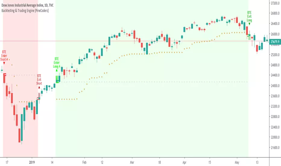
Hellenic EMA Matrix - PremiumHellenic EMA Matrix - Alpha Omega Premium
Complete User Guide
Table of Contents
Introduction
Indicator Philosophy
Mathematical Constants
EMA Types
Settings
Trading Signals
Visualization
Usage Strategies
FAQ
Introduction
Hellenic EMA Matrix is a premium indicator based on mathematical constants of nature: Phi (Phi - Golden Ratio), Pi (Pi), e (Euler's number). The indicator uses these universal constants to create dynamic EMAs that adapt to the natural rhythms of the market.
Key Features:
6 EMA types based on mathematical constants
Premium visualization with Neon Glow and Gradient Clouds
Automatic Fast/Mid/Slow EMA sorting
STRONG signals for powerful trends
Pulsing Ribbon Bar for instant trend assessment
Works on all timeframes (M1 - MN)
Indicator Philosophy
Why Mathematical Constants?
Traditional EMAs use arbitrary periods (9, 21, 50, 200). Hellenic Matrix goes further, using universal mathematical constants found in nature:
Phi (1.618) - Golden Ratio: galaxy spirals, seashells, human body proportions
Pi (3.14159) - Pi: circles, waves, cycles
e (2.71828) - Natural logarithm base: exponential growth, radioactive decay
Markets are also a natural system composed of millions of participants. Using mathematical constants allows tuning into the natural rhythms of market cycles.
Mathematical Constants
Phi (Phi) - Golden Ratio
Phi = 1.618033988749895
Properties:
Phi² = Phi + 1 = 2.618
Phi³ = 4.236
Phi⁴ = 6.854
Application: Ideal for trending movements and Fibonacci corrections
Pi (Pi) - Pi Number
Pi = 3.141592653589793
Properties:
2Pi = 6.283 (full circle)
3Pi = 9.425
4Pi = 12.566
Application: Excellent for cyclical markets and wave structures
e (Euler) - Euler's Number
e = 2.718281828459045
Properties:
e² = 7.389
e³ = 20.085
e⁴ = 54.598
Application: Suitable for exponential movements and volatile markets
EMA Types
1. Phi (Phi) - Golden Ratio EMA
Description: EMA based on the golden ratio
Period Formula:
Period = Phi^n × Base Multiplier
Parameters:
Phi Power Level (1-8): Power of Phi
Phi¹ = 1.618 → ~16 period (with Base=10)
Phi² = 2.618 → ~26 period
Phi³ = 4.236 → ~42 period (recommended)
Phi⁴ = 6.854 → ~69 period
Recommendations:
Phi² or Phi³ for day trading
Phi⁴ or Phi⁵ for swing trading
Works excellently as Fast EMA
2. Pi (Pi) - Circular EMA
Description: EMA based on Pi for cyclical movements
Period Formula:
Period = Pi × Multiple × Base Multiplier
Parameters:
Pi Multiple (1-10): Pi multiplier
1Pi = 3.14 → ~31 period (with Base=10)
2Pi = 6.28 → ~63 period (recommended)
3Pi = 9.42 → ~94 period
Recommendations:
2Pi ideal as Mid or Slow EMA
Excellently identifies cycles and waves
Use on volatile markets (crypto, forex)
3. e (Euler) - Natural EMA
Description: EMA based on natural logarithm
Period Formula:
Period = e^n × Base Multiplier
Parameters:
e Power Level (1-6): Power of e
e¹ = 2.718 → ~27 period (with Base=10)
e² = 7.389 → ~74 period (recommended)
e³ = 20.085 → ~201 period
Recommendations:
e² works excellently as Slow EMA
Ideal for stocks and indices
Filters noise well on lower timeframes
4. Delta (Delta) - Adaptive EMA
Description: Adaptive EMA that changes period based on volatility
Period Formula:
Period = Base Period × (1 + (Volatility - 1) × Factor)
Parameters:
Delta Base Period (5-200): Base period (default 20)
Delta Volatility Sensitivity (0.5-5.0): Volatility sensitivity (default 2.0)
How it works:
During low volatility → period decreases → EMA reacts faster
During high volatility → period increases → EMA smooths noise
Recommendations:
Works excellently on news and sharp movements
Use as Fast EMA for quick adaptation
Sensitivity 2.0-3.0 for crypto, 1.0-2.0 for stocks
5. Sigma (Sigma) - Composite EMA
Description: Composite EMA combining multiple active EMAs
Composition Methods:
Weighted Average (default):
Sigma = (Phi + Pi + e + Delta) / 4
Simple average of all active EMAs
Geometric Mean:
Sigma = fourth_root(Phi × Pi × e × Delta)
Geometric mean (more conservative)
Harmonic Mean:
Sigma = 4 / (1/Phi + 1/Pi + 1/e + 1/Delta)
Harmonic mean (more weight to smaller values)
Recommendations:
Enable for additional confirmation
Use as Mid EMA
Weighted Average - most universal method
6. Lambda (Lambda) - Wave EMA
Description: Wave EMA with sinusoidal period modulation
Period Formula:
Period = Base Period × (1 + Amplitude × sin(2Pi × bar / Frequency))
Parameters:
Lambda Base Period (10-200): Base period
Lambda Wave Amplitude (0.1-2.0): Wave amplitude
Lambda Wave Frequency (10-200): Wave frequency in bars
How it works:
Period pulsates sinusoidally
Creates wave effect following market cycles
Recommendations:
Experimental EMA for advanced users
Works well on cyclical markets
Frequency = 50 for day trading, 100+ for swing
Settings
Matrix Core Settings
Base Multiplier (1-100)
Multiplies all EMA periods
Base = 1: Very fast EMAs (Phi³ = 4, 2Pi = 6, e² = 7)
Base = 10: Standard (Phi³ = 42, 2Pi = 63, e² = 74)
Base = 20: Slow EMAs (Phi³ = 85, 2Pi = 126, e² = 148)
Recommendations by timeframe:
M1-M5: Base = 5-10
M15-H1: Base = 10-15 (recommended)
H4-D1: Base = 15-25
W1-MN: Base = 25-50
Matrix Source
Data source selection for EMA calculation:
close - closing price (standard)
open - opening price
high - high
low - low
hl2 - (high + low) / 2
hlc3 - (high + low + close) / 3
ohlc4 - (open + high + low + close) / 4
When to change:
hlc3 or ohlc4 for smoother signals
high for aggressive longs
low for aggressive shorts
Manual EMA Selection
Critically important setting! Determines which EMAs are used for signal generation.
Use Manual Fast/Slow/Mid Selection
Enabled (default): You select EMAs manually
Disabled: Automatic selection by periods
Fast EMA
Fast EMA - reacts first to price changes
Recommendations:
Phi Golden (recommended) - universal choice
Delta Adaptive - for volatile markets
Must be fastest (smallest period)
Slow EMA
Slow EMA - determines main trend
Recommendations:
Pi Circular (recommended) - excellent trend filter
e Natural - for smoother trend
Must be slowest (largest period)
Mid EMA
Mid EMA - additional signal filter
Recommendations:
e Natural (recommended) - excellent middle level
Pi Circular - alternative
None - for more frequent signals (only 2 EMAs)
IMPORTANT: The indicator automatically sorts selected EMAs by their actual periods:
Fast = EMA with smallest period
Mid = EMA with middle period
Slow = EMA with largest period
Therefore, you can select any combination - the indicator will arrange them correctly!
Premium Visualization
Neon Glow
Enable Neon Glow for EMAs - adds glowing effect around EMA lines
Glow Strength:
Light - subtle glow
Medium (recommended) - optimal balance
Strong - bright glow (may be too bright)
Effect: 2 glow layers around each EMA for 3D effect
Gradient Clouds
Enable Gradient Clouds - fills space between EMAs with gradient
Parameters:
Cloud Transparency (85-98): Cloud transparency
95-97 (recommended)
Higher = more transparent
Dynamic Cloud Intensity - automatically changes transparency based on EMA distance
Cloud Colors:
Phi-Pi Cloud:
Blue - when Pi above Phi (bullish)
Gold - when Phi above Pi (bearish)
Pi-e Cloud:
Green - when e above Pi (bullish)
Blue - when Pi above e (bearish)
2 layers for volumetric effect
Pulsing Ribbon Bar
Enable Pulsing Indicator Bar - pulsing strip at bottom/top of chart
Parameters:
Ribbon Position: Top / Bottom (recommended)
Pulse Speed: Slow / Medium (recommended) / Fast
Symbols and colors:
Green filled square - STRONG BULLISH
Pink filled square - STRONG BEARISH
Blue hollow square - Bullish (regular)
Red hollow square - Bearish (regular)
Purple rectangle - Neutral
Effect: Pulsation with sinusoid for living market feel
Signal Bar Highlights
Enable Signal Bar Highlights - highlights bars with signals
Parameters:
Highlight Transparency (88-96): Highlight transparency
Highlight Style:
Light Fill (recommended) - bar background fill
Thin Line - bar outline only
Highlights:
Golden Cross - green
Death Cross - pink
STRONG BUY - green
STRONG SELL - pink
Show Greek Labels
Shows Greek alphabet letters on last bar:
Phi - Phi EMA (gold)
Pi - Pi EMA (blue)
e - Euler EMA (green)
Delta - Delta EMA (purple)
Sigma - Sigma EMA (pink)
When to use: For education or presentations
Show Old Background
Old background style (not recommended):
Green background - STRONG BULLISH
Pink background - STRONG BEARISH
Blue background - Bullish
Red background - Bearish
Not recommended - use new Gradient Clouds and Pulsing Bar
Info Table
Show Info Table - table with indicator information
Parameters:
Position: Top Left / Top Right (recommended) / Bottom Left / Bottom Right
Size: Tiny / Small (recommended) / Normal / Large
Table contents:
EMA list - periods and current values of all active EMAs
Effects - active visual effects
TREND - current trend state:
STRONG UP - strong bullish
STRONG DOWN - strong bearish
Bullish - regular bullish
Bearish - regular bearish
Neutral - neutral
Momentum % - percentage deviation of price from Fast EMA
Setup - current Fast/Slow/Mid configuration
Trading Signals
Show Golden/Death Cross
Golden Cross - Fast EMA crosses Slow EMA from below (bullish signal) Death Cross - Fast EMA crosses Slow EMA from above (bearish signal)
Symbols:
Yellow dot "GC" below - Golden Cross
Dark red dot "DC" above - Death Cross
Show STRONG Signals
STRONG BUY and STRONG SELL - the most powerful indicator signals
Conditions for STRONG BULLISH:
EMA Alignment: Fast > Mid > Slow (all EMAs aligned)
Trend: Fast > Slow (clear uptrend)
Distance: EMAs separated by minimum 0.15%
Price Position: Price above Fast EMA
Fast Slope: Fast EMA rising
Slow Slope: Slow EMA rising
Mid Trending: Mid EMA also rising (if enabled)
Conditions for STRONG BEARISH:
Same but in reverse
Visual display:
Green label "STRONG BUY" below bar
Pink label "STRONG SELL" above bar
Difference from Golden/Death Cross:
Golden/Death Cross = crossing moment (1 bar)
STRONG signal = sustained trend (lasts several bars)
IMPORTANT: After fixes, STRONG signals now:
Work on all timeframes (M1 to MN)
Don't break on small retracements
Work with any Fast/Mid/Slow combination
Automatically adapt thanks to EMA sorting
Show Stop Loss/Take Profit
Automatic SL/TP level calculation on STRONG signal
Parameters:
Stop Loss (ATR) (0.5-5.0): ATR multiplier for stop loss
1.5 (recommended) - standard
1.0 - tight stop
2.0-3.0 - wide stop
Take Profit R:R (1.0-5.0): Risk/reward ratio
2.0 (recommended) - standard (risk 1.5 ATR, profit 3.0 ATR)
1.5 - conservative
3.0-5.0 - aggressive
Formulas:
LONG:
Stop Loss = Entry - (ATR × Stop Loss ATR)
Take Profit = Entry + (ATR × Stop Loss ATR × Take Profit R:R)
SHORT:
Stop Loss = Entry + (ATR × Stop Loss ATR)
Take Profit = Entry - (ATR × Stop Loss ATR × Take Profit R:R)
Visualization:
Red X - Stop Loss
Green X - Take Profit
Levels remain active while STRONG signal persists
Trading Signals
Signal Types
1. Golden Cross
Description: Fast EMA crosses Slow EMA from below
Signal: Beginning of bullish trend
How to trade:
ENTRY: On bar close with Golden Cross
STOP: Below local low or below Slow EMA
TARGET: Next resistance level or 2:1 R:R
Strengths:
Simple and clear
Works well on trending markets
Clear entry point
Weaknesses:
Lags (signal after movement starts)
Many false signals in ranging markets
May be late on fast moves
Optimal timeframes: H1, H4, D1
2. Death Cross
Description: Fast EMA crosses Slow EMA from above
Signal: Beginning of bearish trend
How to trade:
ENTRY: On bar close with Death Cross
STOP: Above local high or above Slow EMA
TARGET: Next support level or 2:1 R:R
Application: Mirror of Golden Cross
3. STRONG BUY
Description: All EMAs aligned + trend + all EMAs rising
Signal: Powerful bullish trend
How to trade:
ENTRY: On bar close with STRONG BUY or on pullback to Fast EMA
STOP: Below Fast EMA or automatic SL (if enabled)
TARGET: Automatic TP (if enabled) or by levels
TRAILING: Follow Fast EMA
Entry strategies:
Aggressive: Enter immediately on signal
Conservative: Wait for pullback to Fast EMA, then enter on bounce
Pyramiding: Add positions on pullbacks to Mid EMA
Position management:
Hold while STRONG signal active
Exit on STRONG SELL or Death Cross appearance
Move stop behind Fast EMA
Strengths:
Most reliable indicator signal
Doesn't break on pullbacks
Catches large moves
Works on all timeframes
Weaknesses:
Appears less frequently than other signals
Requires confirmation (multiple conditions)
Optimal timeframes: All (M5 - D1)
4. STRONG SELL
Description: All EMAs aligned down + downtrend + all EMAs falling
Signal: Powerful bearish trend
How to trade: Mirror of STRONG BUY
Visual Signals
Pulsing Ribbon Bar
Quick market assessment at a glance:
Symbol Color State
Filled square Green STRONG BULLISH
Filled square Pink STRONG BEARISH
Hollow square Blue Bullish
Hollow square Red Bearish
Rectangle Purple Neutral
Pulsation: Sinusoidal, creates living effect
Signal Bar Highlights
Bars with signals are highlighted:
Green highlight: STRONG BUY or Golden Cross
Pink highlight: STRONG SELL or Death Cross
Gradient Clouds
Colored space between EMAs shows trend strength:
Wide clouds - strong trend
Narrow clouds - weak trend or consolidation
Color change - trend change
Info Table
Quick reference in corner:
TREND: Current state (STRONG UP, Bullish, Neutral, Bearish, STRONG DOWN)
Momentum %: Movement strength
Effects: Active visual effects
Setup: Fast/Slow/Mid configuration
Usage Strategies
Strategy 1: "Golden Trailing"
Idea: Follow STRONG signals using Fast EMA as trailing stop
Settings:
Fast: Phi Golden (Phi³)
Mid: Pi Circular (2Pi)
Slow: e Natural (e²)
Base Multiplier: 10
Timeframe: H1, H4
Entry rules:
Wait for STRONG BUY
Enter on bar close or on pullback to Fast EMA
Stop below Fast EMA
Management:
Hold position while STRONG signal active
Move stop behind Fast EMA daily
Exit on STRONG SELL or Death Cross
Take Profit:
Partially close at +2R
Trail remainder until exit signal
For whom: Swing traders, trend followers
Pros:
Catches large moves
Simple rules
Emotionally comfortable
Cons:
Requires patience
Possible extended drawdowns on pullbacks
Strategy 2: "Scalping Bounces"
Idea: Scalp bounces from Fast EMA during STRONG trend
Settings:
Fast: Delta Adaptive (Base 15, Sensitivity 2.0)
Mid: Phi Golden (Phi²)
Slow: Pi Circular (2Pi)
Base Multiplier: 5
Timeframe: M5, M15
Entry rules:
STRONG signal must be active
Wait for price pullback to Fast EMA
Enter on bounce (candle closes above/below Fast EMA)
Stop behind local extreme (15-20 pips)
Take Profit:
+1.5R or to Mid EMA
Or to next level
For whom: Active day traders
Pros:
Many signals
Clear entry point
Quick profits
Cons:
Requires constant monitoring
Not all bounces work
Requires discipline for frequent trading
Strategy 3: "Triple Filter"
Idea: Enter only when all 3 EMAs and price perfectly aligned
Settings:
Fast: Phi Golden (Phi³)
Mid: e Natural (e²)
Slow: Pi Circular (3Pi)
Base Multiplier: 15
Timeframe: H4, D1
Entry rules (LONG):
STRONG BUY active
Price above all three EMAs
Fast > Mid > Slow (all aligned)
All EMAs rising (slope up)
Gradient Clouds wide and bright
Entry:
On bar close meeting all conditions
Or on next pullback to Fast EMA
Stop:
Below Mid EMA or -1.5 ATR
Take Profit:
First target: +3R
Second target: next major level
Trailing: Mid EMA
For whom: Conservative swing traders, investors
Pros:
Very reliable signals
Minimum false entries
Large profit potential
Cons:
Rare signals (2-5 per month)
Requires patience
Strategy 4: "Adaptive Scalper"
Idea: Use only Delta Adaptive EMA for quick volatility reaction
Settings:
Fast: Delta Adaptive (Base 10, Sensitivity 3.0)
Mid: None
Slow: Delta Adaptive (Base 30, Sensitivity 2.0)
Base Multiplier: 3
Timeframe: M1, M5
Feature: Two different Delta EMAs with different settings
Entry rules:
Golden Cross between two Delta EMAs
Both Delta EMAs must be rising/falling
Enter on next bar
Stop:
10-15 pips or below Slow Delta EMA
Take Profit:
+1R to +2R
Or Death Cross
For whom: Scalpers on cryptocurrencies and forex
Pros:
Instant volatility adaptation
Many signals on volatile markets
Quick results
Cons:
Much noise on calm markets
Requires fast execution
High commissions may eat profits
Strategy 5: "Cyclical Trader"
Idea: Use Pi and Lambda for trading cyclical markets
Settings:
Fast: Pi Circular (1Pi)
Mid: Lambda Wave (Base 30, Amplitude 0.5, Frequency 50)
Slow: Pi Circular (3Pi)
Base Multiplier: 10
Timeframe: H1, H4
Entry rules:
STRONG signal active
Lambda Wave EMA synchronized with trend
Enter on bounce from Lambda Wave
For whom: Traders of cyclical assets (some altcoins, commodities)
Pros:
Catches cyclical movements
Lambda Wave provides additional entry points
Cons:
More complex to configure
Not for all markets
Lambda Wave may give false signals
Strategy 6: "Multi-Timeframe Confirmation"
Idea: Use multiple timeframes for confirmation
Scheme:
Higher TF (D1): Determine trend direction (STRONG signal)
Middle TF (H4): Wait for STRONG signal in same direction
Lower TF (M15): Look for entry point (Golden Cross or bounce from Fast EMA)
Settings for all TFs:
Fast: Phi Golden (Phi³)
Mid: e Natural (e²)
Slow: Pi Circular (2Pi)
Base Multiplier: 10
Rules:
All 3 TFs must show one trend
Entry on lower TF
Stop by lower TF
Target by higher TF
For whom: Serious traders and investors
Pros:
Maximum reliability
Large profit targets
Minimum false signals
Cons:
Rare setups
Requires analysis of multiple charts
Experience needed
Practical Tips
DOs
Use STRONG signals as primary - they're most reliable
Let signals develop - don't exit on first pullback
Use trailing stop - follow Fast EMA
Combine with levels - S/R, Fibonacci, volumes
Test on demo before real
Adjust Base Multiplier for your timeframe
Enable visual effects - they help see the picture
Use Info Table - quick situation assessment
Watch Pulsing Bar - instant state indicator
Trust auto-sorting of Fast/Mid/Slow
DON'Ts
Don't trade against STRONG signal - trend is your friend
Don't ignore Mid EMA - it adds reliability
Don't use too small Base Multiplier on higher TFs
Don't enter on Golden Cross in range - check for trend
Don't change settings during open position
Don't forget risk management - 1-2% per trade
Don't trade all signals in row - choose best ones
Don't use indicator in isolation - combine with Price Action
Don't set too tight stops - let trade breathe
Don't over-optimize - simplicity = reliability
Optimal Settings by Asset
US Stocks (SPY, AAPL, TSLA)
Recommendation:
Fast: Phi Golden (Phi³)
Mid: e Natural (e²)
Slow: Pi Circular (2Pi)
Base: 10-15
Timeframe: H4, D1
Features:
Use on daily for swing
STRONG signals very reliable
Works well on trending stocks
Forex (EUR/USD, GBP/USD)
Recommendation:
Fast: Delta Adaptive (Base 15, Sens 2.0)
Mid: Phi Golden (Phi²)
Slow: Pi Circular (2Pi)
Base: 8-12
Timeframe: M15, H1, H4
Features:
Delta Adaptive works excellently on news
Many signals on M15-H1
Consider spreads
Cryptocurrencies (BTC, ETH, altcoins)
Recommendation:
Fast: Delta Adaptive (Base 10, Sens 3.0)
Mid: Pi Circular (2Pi)
Slow: e Natural (e²)
Base: 5-10
Timeframe: M5, M15, H1
Features:
High volatility - adaptation needed
STRONG signals can last days
Be careful with scalping on M1-M5
Commodities (Gold, Oil)
Recommendation:
Fast: Pi Circular (1Pi)
Mid: Phi Golden (Phi³)
Slow: Pi Circular (3Pi)
Base: 12-18
Timeframe: H4, D1
Features:
Pi works excellently on cyclical commodities
Gold responds especially well to Phi
Oil volatile - use wide stops
Indices (S&P500, Nasdaq, DAX)
Recommendation:
Fast: Phi Golden (Phi³)
Mid: e Natural (e²)
Slow: Pi Circular (2Pi)
Base: 15-20
Timeframe: H4, D1, W1
Features:
Very trending instruments
STRONG signals last weeks
Good for position trading
Alerts
The indicator supports 6 alert types:
1. Golden Cross
Message: "Hellenic Matrix: GOLDEN CROSS - Fast EMA crossed above Slow EMA - Bullish trend starting!"
When: Fast EMA crosses Slow EMA from below
2. Death Cross
Message: "Hellenic Matrix: DEATH CROSS - Fast EMA crossed below Slow EMA - Bearish trend starting!"
When: Fast EMA crosses Slow EMA from above
3. STRONG BULLISH
Message: "Hellenic Matrix: STRONG BULLISH SIGNAL - All EMAs aligned for powerful uptrend!"
When: All conditions for STRONG BUY met (first bar)
4. STRONG BEARISH
Message: "Hellenic Matrix: STRONG BEARISH SIGNAL - All EMAs aligned for powerful downtrend!"
When: All conditions for STRONG SELL met (first bar)
5. Bullish Ribbon
Message: "Hellenic Matrix: BULLISH RIBBON - EMAs aligned for uptrend"
When: EMAs aligned bullish + price above Fast EMA (less strict condition)
6. Bearish Ribbon
Message: "Hellenic Matrix: BEARISH RIBBON - EMAs aligned for downtrend"
When: EMAs aligned bearish + price below Fast EMA (less strict condition)
How to Set Up Alerts:
Open indicator on chart
Click on three dots next to indicator name
Select "Create Alert"
In "Condition" field select needed alert:
Golden Cross
Death Cross
STRONG BULLISH
STRONG BEARISH
Bullish Ribbon
Bearish Ribbon
Configure notification method:
Pop-up in browser
Email
SMS (in Premium accounts)
Push notifications in mobile app
Webhook (for automation)
Select frequency:
Once Per Bar Close (recommended) - once on bar close
Once Per Bar - during bar formation
Only Once - only first time
Click "Create"
Tip: Create separate alerts for different timeframes and instruments
FAQ
1. Why don't STRONG signals appear?
Possible reasons:
Incorrect Fast/Mid/Slow order
Solution: Indicator automatically sorts EMAs by periods, but ensure selected EMAs have different periods
Base Multiplier too large
Solution: Reduce Base to 5-10 on lower timeframes
Market in range
Solution: STRONG signals appear only in trends - this is normal
Too strict EMA settings
Solution: Try classic combination: Phi³ / Pi×2 / e² with Base=10
Mid EMA too close to Fast or Slow
Solution: Select Mid EMA with period between Fast and Slow
2. How often should STRONG signals appear?
Normal frequency:
M1-M5: 5-15 signals per day (very active markets)
M15-H1: 2-8 signals per day
H4: 3-10 signals per week
D1: 2-5 signals per month
W1: 2-6 signals per year
If too many signals - market very volatile or Base too small
If too few signals - market in range or Base too large
4. What are the best settings for beginners?
Universal "out of the box" settings:
Matrix Core:
Base Multiplier: 10
Source: close
Phi Golden: Enabled, Power = 3
Pi Circular: Enabled, Multiple = 2
e Natural: Enabled, Power = 2
Delta Adaptive: Enabled, Base = 20, Sensitivity = 2.0
Manual Selection:
Fast: Phi Golden
Mid: e Natural
Slow: Pi Circular
Visualization:
Gradient Clouds: ON
Neon Glow: ON (Medium)
Pulsing Bar: ON (Medium)
Signal Highlights: ON (Light Fill)
Table: ON (Top Right, Small)
Signals:
Golden/Death Cross: ON
STRONG Signals: ON
Stop Loss: OFF (while learning)
Timeframe for learning: H1 or H4
5. Can I use only one EMA?
No, minimum 2 EMAs (Fast and Slow) for signal generation.
Mid EMA is optional:
With Mid EMA = more reliable but rarer signals
Without Mid EMA = more signals but less strict filtering
Recommendation: Start with 3 EMAs (Fast/Mid/Slow), then experiment
6. Does the indicator work on cryptocurrencies?
Yes, works excellently! Especially good on:
Bitcoin (BTC)
Ethereum (ETH)
Major altcoins (SOL, BNB, XRP)
Recommended settings for crypto:
Fast: Delta Adaptive (Base 10-15, Sensitivity 2.5-3.0)
Mid: Pi Circular (2Pi)
Slow: e Natural (e²)
Base: 5-10
Timeframe: M15, H1, H4
Crypto market features:
High volatility → use Delta Adaptive
24/7 trading → set alerts
Sharp movements → wide stops
7. Can I trade only with this indicator?
Technically yes, but NOT recommended.
Best approach - combine with:
Price Action - support/resistance levels, candle patterns
Volume - movement strength confirmation
Fibonacci - retracement and extension levels
RSI/MACD - divergences and overbought/oversold
Fundamental analysis - news, company reports
Hellenic Matrix:
Excellently determines trend and its strength
Provides clear entry/exit points
Doesn't consider fundamentals
Doesn't see major levels
8. Why do Gradient Clouds change color?
Color depends on EMA order:
Phi-Pi Cloud:
Blue - Pi EMA above Phi EMA (bullish alignment)
Gold - Phi EMA above Pi EMA (bearish alignment)
Pi-e Cloud:
Green - e EMA above Pi EMA (bullish alignment)
Blue - Pi EMA above e EMA (bearish alignment)
Color change = EMA order change = possible trend change
9. What is Momentum % in the table?
Momentum % = percentage deviation of price from Fast EMA
Formula:
Momentum = ((Close - Fast EMA) / Fast EMA) × 100
Interpretation:
+0.5% to +2% - normal bullish momentum
+2% to +5% - strong bullish momentum
+5% and above - overheating (correction possible)
-0.5% to -2% - normal bearish momentum
-2% to -5% - strong bearish momentum
-5% and below - oversold (bounce possible)
Usage:
Monitor momentum during STRONG signals
Large momentum = don't enter (wait for pullback)
Small momentum = good entry point
10. How to configure for scalping?
Settings for scalping (M1-M5):
Base Multiplier: 3-5
Source: close or hlc3 (smoother)
Fast: Delta Adaptive (Base 8-12, Sensitivity 3.0)
Mid: None (for more signals)
Slow: Phi Golden (Phi²) or Pi Circular (1Pi)
Visualization:
- Gradient Clouds: ON (helps see strength)
- Neon Glow: OFF (doesn't clutter chart)
- Pulsing Bar: ON (quick assessment)
- Signal Highlights: ON
Signals:
- Golden/Death Cross: ON
- STRONG Signals: ON
- Stop Loss: ON (1.0-1.5 ATR, R:R 1.5-2.0)
Scalping rules:
Trade only STRONG signals
Enter on bounce from Fast EMA
Tight stops (10-20 pips)
Quick take profit (+1R to +2R)
Don't hold through news
11. How to configure for long-term investing?
Settings for investing (D1-W1):
Base Multiplier: 20-30
Source: close
Fast: Phi Golden (Phi³ or Phi⁴)
Mid: e Natural (e²)
Slow: Pi Circular (3Pi or 4Pi)
Visualization:
- Gradient Clouds: ON
- Neon Glow: ON (Medium)
- Everything else - to taste
Signals:
- Golden/Death Cross: ON
- STRONG Signals: ON
- Stop Loss: OFF (use percentage stop)
Investing rules:
Enter only on STRONG signals
Hold while STRONG active (weeks/months)
Stop below Slow EMA or -10%
Take profit: by company targets or +50-100%
Ignore short-term pullbacks
12. What if indicator slows down chart?
Indicator is optimized, but if it slows:
Disable unnecessary visual effects:
Neon Glow: OFF (saves 8 plots)
Gradient Clouds: ON but low quality
Lambda Wave EMA: OFF (if not using)
Reduce number of active EMAs:
Sigma Composite: OFF
Lambda Wave: OFF
Leave only Phi, Pi, e, Delta
Simplify settings:
Pulsing Bar: OFF
Greek Labels: OFF
Info Table: smaller size
13. Can I use on different timeframes simultaneously?
Yes! Multi-timeframe analysis is very powerful:
Classic scheme:
Higher TF (D1, W1) - determine global trend
Wait for STRONG signal
This is our trading direction
Middle TF (H4, H1) - look for confirmation
STRONG signal in same direction
Precise entry zone
Lower TF (M15, M5) - entry point
Golden Cross or bounce from Fast EMA
Precise stop loss
Example:
W1: STRONG BUY active (global uptrend)
H4: STRONG BUY appeared (confirmation)
M15: Wait for Golden Cross or bounce from Fast EMA → ENTRY
Advantages:
Maximum reliability
Clear timeframe hierarchy
Large targets
14. How does indicator work on news?
Delta Adaptive EMA adapts excellently to news:
Before news:
Low volatility → Delta EMA becomes fast → pulls to price
During news:
Sharp volatility spike → Delta EMA slows → filters noise
After news:
Volatility normalizes → Delta EMA returns to normal
Recommendations:
Don't trade at news release moment (spreads widen)
Wait for STRONG signal after news (2-5 bars)
Use Delta Adaptive as Fast EMA for quick reaction
Widen stops by 50-100% during important news
Advanced Techniques
Technique 1: "Divergences with EMA"
Idea: Look for discrepancies between price and Fast EMA
Bullish divergence:
Price makes lower low
Fast EMA makes higher low
= Possible reversal up
Bearish divergence:
Price makes higher high
Fast EMA makes lower high
= Possible reversal down
How to trade:
Find divergence
Wait for STRONG signal in divergence direction
Enter on confirmation
Technique 2: "EMA Tunnel"
Idea: Use space between Fast and Slow EMA as "tunnel"
Rules:
Wide tunnel - strong trend, hold position
Narrow tunnel - weak trend or consolidation, caution
Tunnel narrowing - trend weakening, prepare to exit
Tunnel widening - trend strengthening, can add
Visually: Gradient Clouds show this automatically!
Trading:
Enter on STRONG signal (tunnel starts widening)
Hold while tunnel wide
Exit when tunnel starts narrowing
Technique 3: "Wave Analysis with Lambda"
Idea: Lambda Wave EMA creates sinusoid matching market cycles
Setup:
Lambda Base Period: 30
Lambda Wave Amplitude: 0.5
Lambda Wave Frequency: 50 (adjusted to asset cycle)
How to find correct Frequency:
Look at historical cycles (distance between local highs)
Average distance = your Frequency
Example: if highs every 40-60 bars, set Frequency = 50
Trading:
Enter when Lambda Wave at bottom of sinusoid (growth potential)
Exit when Lambda Wave at top (fall potential)
Combine with STRONG signals
Technique 4: "Cluster Analysis"
Idea: When all EMAs gather in narrow cluster = powerful breakout soon
Cluster signs:
All EMAs (Phi, Pi, e, Delta) within 0.5-1% of each other
Gradient Clouds almost invisible
Price jumping around all EMAs
Trading:
Identify cluster (all EMAs close)
Determine breakout direction (where more volume, higher TFs direction)
Wait for breakout and STRONG signal
Enter on confirmation
Target = cluster size × 3-5
This is very powerful technique for big moves!
Technique 5: "Sigma as Dynamic Level"
Idea: Sigma Composite EMA = average of all EMAs = magnetic level
Usage:
Enable Sigma Composite (Weighted Average)
Sigma works as dynamic support/resistance
Price often returns to Sigma before trend continuation
Trading:
In trend: Enter on bounces from Sigma
In range: Fade moves from Sigma (trade return to Sigma)
On breakout: Sigma becomes support/resistance
Risk Management
Basic Rules
1. Position Size
Conservative: 1% of capital per trade
Moderate: 2% of capital per trade (recommended)
Aggressive: 3-5% (only for experienced)
Calculation formula:
Lot Size = (Capital × Risk%) / (Stop in pips × Pip value)
2. Risk/Reward Ratio
Minimum: 1:1.5
Standard: 1:2 (recommended)
Optimal: 1:3
Aggressive: 1:5+
3. Maximum Drawdown
Daily: -3% to -5%
Weekly: -7% to -10%
Monthly: -15% to -20%
Upon reaching limit → STOP trading until end of period
Position Management Strategies
1. Fixed Stop
Method:
Stop below/above Fast EMA or local extreme
DON'T move stop against position
Can move to breakeven
For whom: Beginners, conservative traders
2. Trailing by Fast EMA
Method:
Each day (or bar) move stop to Fast EMA level
Position closes when price breaks Fast EMA
Advantages:
Stay in trend as long as possible
Automatically exit on reversal
For whom: Trend followers, swing traders
3. Partial Exit
Method:
50% of position close at +2R
50% hold with trailing by Mid EMA or Slow EMA
Advantages:
Lock profit
Leave position for big move
Psychologically comfortable
For whom: Universal method (recommended)
4. Pyramiding
Method:
First entry on STRONG signal (50% of planned position)
Add 25% on pullback to Fast EMA
Add another 25% on pullback to Mid EMA
Overall stop below Slow EMA
Advantages:
Average entry price
Reduce risk
Increase profit in strong trends
Caution:
Works only in trends
In range leads to losses
For whom: Experienced traders
Trading Psychology
Correct Mindset
1. Indicator is a tool, not holy grail
Indicator shows probability, not guarantee
There will be losing trades - this is normal
Important is series statistics, not one trade
2. Trust the system
If STRONG signal appeared - enter
Don't search for "perfect" moment
Follow trading plan
3. Patience
STRONG signals don't appear every day
Better miss signal than enter against trend
Quality over quantity
4. Discipline
Always set stop loss
Don't move stop against position
Don't increase risk after losses
Beginner Mistakes
1. "I know better than indicator"
Indicator says STRONG BUY, but you think "too high, will wait for pullback"
Result: miss profitable move
Solution: Trust signals or don't use indicator
2. "Will reverse now for sure"
Trading against STRONG trend
Result: stops, stops, stops
Solution: Trend is your friend, trade with trend
3. "Will hold a bit more"
Don't exit when STRONG signal disappears
Greed eats profit
Solution: If signal gone - exit!
4. "I'll recover"
After losses double risk
Result: huge losses
Solution: Fixed % risk ALWAYS
5. "I don't like this signal"
Skip signals because of "feeling"
Result: inconsistency, no statistics
Solution: Trade ALL signals or clearly define filters
Trading Journal
What to Record
For each trade:
1. Entry/exit date and time
2. Instrument and timeframe
3. Signal type
Golden Cross
STRONG BUY
STRONG SELL
Death Cross
4. Indicator settings
Fast/Mid/Slow EMA
Base Multiplier
Other parameters
5. Chart screenshot
Entry moment
Exit moment
6. Trade parameters
Position size
Stop loss
Take Profit
R:R
7. Result
Profit/Loss in $
Profit/Loss in %
Profit/Loss in R
8. Notes
What was right
What was wrong
Emotions during trade
Lessons
Journal Analysis
Analyze weekly:
1. Win Rate
Win Rate = (Profitable trades / All trades) × 100%
Good: 50-60%
Excellent: 60-70%
Exceptional: 70%+
2. Average R
Average R = Sum of all R / Number of trades
Good: +0.5R
Excellent: +1.0R
Exceptional: +1.5R+
3. Profit Factor
Profit Factor = Total profit / Total losses
Good: 1.5+
Excellent: 2.0+
Exceptional: 3.0+
4. Maximum Drawdown
Track consecutive losses
If more than 5 in row - stop, check system
5. Best/Worst Trades
What was common in best trades? (do more)
What was common in worst trades? (avoid)
Pre-Trade Checklist
Technical Analysis
STRONG signal active (BUY or SELL)
All EMAs properly aligned (Fast > Mid > Slow or reverse)
Price on correct side of Fast EMA
Gradient Clouds confirm trend
Pulsing Bar shows STRONG state
Momentum % in normal range (not overheated)
No close strong levels against direction
Higher timeframe doesn't contradict
Risk Management
Position size calculated (1-2% risk)
Stop loss set
Take profit calculated (minimum 1:2)
R:R satisfactory
Daily/weekly risk limit not exceeded
No other open correlated positions
Fundamental Analysis
No important news in coming hours
Market session appropriate (liquidity)
No contradicting fundamentals
Understand why asset is moving
Psychology
Calm and thinking clearly
No emotions from previous trades
Ready to accept loss at stop
Following trading plan
Not revenging market for past losses
If at least one point is NO - think twice before entering!
Learning Roadmap
Week 1: Familiarization
Goals:
Install and configure indicator
Study all EMA types
Understand visualization
Tasks:
Add indicator to chart
Test all Fast/Mid/Slow settings
Play with Base Multiplier on different timeframes
Observe Gradient Clouds and Pulsing Bar
Study Info Table
Result: Comfort with indicator interface
Week 2: Signals
Goals:
Learn to recognize all signal types
Understand difference between Golden Cross and STRONG
Tasks:
Find 10 Golden Cross examples in history
Find 10 STRONG BUY examples in history
Compare their results (which worked better)
Set up alerts
Get 5 real alerts
Result: Understanding signals
Week 3: Demo Trading
Goals:
Start trading signals on demo account
Gather statistics
Tasks:
Open demo account
Trade ONLY STRONG signals
Keep journal (minimum 20 trades)
Don't change indicator settings
Strictly follow stop losses
Result: 20+ documented trades
Week 4: Analysis
Goals:
Analyze demo trading results
Optimize approach
Tasks:
Calculate win rate and average R
Find patterns in profitable trades
Find patterns in losing trades
Adjust approach (not indicator!)
Write trading plan
Result: Trading plan on 1 page
Month 2: Improvement
Goals:
Deepen understanding
Add additional techniques
Tasks:
Study multi-timeframe analysis
Test combinations with Price Action
Try advanced techniques (divergences, tunnels)
Continue demo trading (minimum 50 trades)
Achieve stable profitability on demo
Result: Win rate 55%+ and Profit Factor 1.5+
Month 3: Real Trading
Goals:
Transition to real account
Maintain discipline
Tasks:
Open small real account
Trade minimum lots
Strictly follow trading plan
DON'T increase risk
Focus on process, not profit
Result: Psychological comfort on real
Month 4+: Scaling
Goals:
Increase account
Become consistently profitable
Tasks:
With 60%+ win rate can increase risk to 2%
Upon doubling account can add capital
Continue keeping journal
Periodically review and improve strategy
Share experience with community
Result: Stable profitability month after month
Additional Resources
Recommended Reading
Technical Analysis:
"Technical Analysis of Financial Markets" - John Murphy
"Trading in the Zone" - Mark Douglas (psychology)
"Market Wizards" - Jack Schwager (trader interviews)
EMA and Moving Averages:
"Moving Averages 101" - Steve Burns
Articles on Investopedia about EMA
Risk Management:
"The Mathematics of Money Management" - Ralph Vince
"Trade Your Way to Financial Freedom" - Van K. Tharp
Trading Journals:
Edgewonk (paid, very powerful)
Tradervue (free version + premium)
Excel/Google Sheets (free)
Screeners:
TradingView Stock Screener
Finviz (stocks)
CoinMarketCap (crypto)
Conclusion
Hellenic EMA Matrix is a powerful tool based on universal mathematical constants of nature. The indicator combines:
Mathematical elegance - Phi, Pi, e instead of arbitrary numbers
Premium visualization - Neon Glow, Gradient Clouds, Pulsing Bar
Reliable signals - STRONG BUY/SELL work on all timeframes
Flexibility - 6 EMA types, adaptation to any trading style
Automation - auto-sorting EMAs, SL/TP calculation, alerts
Key Success Principles:
Simplicity - start with basic settings (Phi/Pi/e, Base=10)
Discipline - follow STRONG signals strictly
Patience - wait for quality setups
Risk Management - 1-2% per trade, ALWAYS
Journal - document every trade
Learning - constantly improve skills
Remember:
Indicator shows probability, not guarantee
Important is series statistics, not one trade
Psychology more important than technique
Quality more important than quantity
Process more important than result
Acknowledgments
Thank you for using Hellenic EMA Matrix - Alpha Omega Premium!
The indicator was created with love for mathematics, markets, and beautiful visualization.
Wishing you profitable trading!
Guide Version: 1.0
Date: 2025
Compatibility: Pine Script v6, TradingView
"In the simplicity of mathematical constants lies the complexity of market movements"

GKD-C Adaptive-Lookback Phase Change Index [Loxx]Giga Kaleidoscope GKD-C Adaptive-Lookback Phase Change Index is a Confirmation module included in Loxx's "Giga Kaleidoscope Modularized Trading System".
█ GKD-C Adaptive-Lookback Phase Change Index
What is the Phase Change Index?
The Phase Change Index (PCI) is a technical indicator that has gained popularity among traders in recent years. It is used to identify market phases and make profitable trades based on momentum and price data. The PCI was developed by M.H. Pee and first introduced in the Stocks & Commodities magazine in 2004.
The PCI is calculated using the 35-day momentum and the 35-day price channel index (PCI). The momentum is the difference between the current day's close and the close 35 days ago, while the PCI measures the distance between the highest high and lowest low over a period of 35 days. By combining these two indicators, traders can identify six possible market phases, each with its own trading strategy.
The formula for calculating the Phase Change Index (PCI) is as follows:
PCI = 100 * (C - L) / (H - L)
Where:
- C is the closing price of the current day
- L is the lowest low over a period of 35 days
- H is the highest high over a period of 35 days
The formula for calculating momentum is as follows:
Momentum = C - Cn
Where:
- C is the closing price of the current day
- Cn is the closing price n days ago, where n = 35 in this case.
The first two phases are characterized by negative momentum, with phase one having a low PCI value (less than 20) and phase two having a high PCI value (greater than 80). In these phases, traders should enter short positions. The next two phases have positive momentum, with phase three having a low PCI value and phase four having a high PCI value. In these phases, traders should enter long positions.
The final two phases are characterized by neutral momentum, with phase five having a low PCI value and phase six having a high PCI value. In these phases, traders should maintain their previous positions until there is a clear signal to enter or exit.
Traders can also use other technical indicators in conjunction with the PCI to confirm signals or filter out false signals. For example, some traders use moving averages or trendlines to confirm trend direction before entering a trade based on the PCI.
In conclusion, the Phase Change Index is a powerful technical indicator that can help traders identify market phases and make profitable trades. By combining momentum and price data, traders can enter long or short positions based on the six possible market phases. Backtesting results have shown that the PCI is robust across parameters, markets, and years. However, it is important to use proper risk management and not rely solely on past profitability when making trading decisions.
What is the Jurik Filter?
The Jurik Filter is a technical analysis tool that is used to filter out market noise and identify trends in financial markets. It was developed by Mark Jurik in the 1990s and is based on a non-linear smoothing algorithm that provides a more accurate representation of price movements.
Traditional moving averages, such as the Simple Moving Average ( SMA ) or Exponential Moving Average ( EMA ), are linear filters that produce a lag between price and the moving average line. This can cause false signals during periods of market volatility , which can result in losses for traders and investors.
The Jurik Filter is designed to address this issue by incorporating a damping factor into the smoothing algorithm. This damping factor adjusts the filter's responsiveness to the changes in price, allowing it to filter out market noise without overshooting price peaks and valleys.
The Jurik Filter is calculated using a mathematical formula that takes into account the current and past prices of an asset, as well as the volatility of the market. This formula incorporates the damping factor and produces a smoother price curve than traditional moving average filters.
One of the advantages of the Jurik Filter is its ability to adjust to changing market conditions. The damping factor can be adjusted to suit different securities and time frames, making it a versatile tool for traders and investors.
Traders and investors often use the Jurik Filter in conjunction with other technical analysis tools, such as the MACD or RSI , to confirm or complement their trading strategies. By filtering out market noise and identifying trends in the financial markets, the Jurik Filter can help improve the accuracy of trading signals and reduce the risks of false signals during periods of market volatility .
Overall, the Jurik Filter is a powerful technical analysis tool that can help traders and investors make more informed decisions about buying and selling securities. By providing a smoother price curve and reducing false signals, it can help improve trading performance and reduce risk in volatile markets.
What is the Adaptive Lookback Period?
The adaptive lookback period is a technique used in technical analysis to adjust the period of an indicator based on changes in market conditions. This technique is particularly useful in volatile or rapidly changing markets where a fixed period may not be optimal for detecting trends or signals.
The concept of the adaptive lookback period is relatively simple. By adjusting the lookback period based on changes in market conditions, traders can more accurately identify trends and signals. This can help traders to enter and exit trades at the right time and improve the profitability of their trading strategies.
The adaptive lookback period works by identifying potential swing points in the market. Once these points are identified, the lookback period is calculated based on the number of swings and a speed parameter. The swing count parameter determines the number of swings that must occur before the lookback period is adjusted. The speed parameter controls the rate at which the lookback period is adjusted, with higher values indicating a more rapid adjustment.
The adaptive lookback period can be applied to a wide range of technical indicators, including moving averages, oscillators, and trendlines. By adjusting the period of these indicators based on changes in market conditions, traders can reduce the impact of noise and false signals, leading to more profitable trades.
In summary, the adaptive lookback period is a powerful technique for traders and analysts looking to optimize their technical indicators. By adjusting the period based on changes in market conditions, traders can more accurately identify trends and signals, leading to more profitable trades. While there are various ways to implement the adaptive lookback period, the basic concept remains the same, and traders can adapt and customize the technique to suit their individual needs and trading styles.
What is the Adaptive-Lookback Phase Change Index?
The combination of adaptive lookback and Jurik filtering is an effective technique used in technical analysis to filter out market noise and improve the accuracy of trading signals. When applied to the Phase Change Index (PCI) indicator, the adaptive lookback period can be used to adjust the period of the indicator based on changes in market conditions. Jurik filtering can then be used to filter out market noise and improve the accuracy of the signals produced by the PCI indicator.
The adaptive lookback period is particularly useful in volatile or rapidly changing markets where a fixed period may not be optimal for detecting trends or signals. By adjusting the lookback period based on changes in market conditions, traders can more accurately identify trends and signals, leading to more profitable trades.
Jurik filtering is a more advanced filtering technique that uses a combination of smoothing and phase shift to produce a more accurate signal. This technique is particularly useful in filtering out market noise and improving the accuracy of trading signals. Jurik filtering can be applied to various indicators, including moving averages, oscillators, and trendlines.
Overall, the combination of adaptive lookback and Jurik filtering is a powerful technique used in technical analysis to filter out market noise and improve the accuracy of trading signals. When applied to the Phase Change Index (PCI) indicator, this technique is particularly effective in identifying trend changes and producing more accurate signals for entry and exit points in trading strategies.
Keep in mind, this is an inverse indicator meaning that above the middle-line/signal is short, below is long.
Additional Features
This indicator allows you to select from 33 source types. They are as follows:
Close
Open
High
Low
Median
Typical
Weighted
Average
Average Median Body
Trend Biased
Trend Biased (Extreme)
HA Close
HA Open
HA High
HA Low
HA Median
HA Typical
HA Weighted
HA Average
HA Average Median Body
HA Trend Biased
HA Trend Biased (Extreme)
HAB Close
HAB Open
HAB High
HAB Low
HAB Median
HAB Typical
HAB Weighted
HAB Average
HAB Average Median Body
HAB Trend Biased
HAB Trend Biased (Extreme)
What are Heiken Ashi "better" candles?
Heiken Ashi "better" candles are a modified version of the standard Heiken Ashi candles, which are a popular charting technique used in technical analysis. Heiken Ashi candles help traders identify trends and potential reversal points by smoothing out price data and reducing market noise. The "better formula" was proposed by Sebastian Schmidt in an article published by BNP Paribas in Warrants & Zertifikate, a German magazine, in August 2004. The aim of this formula is to further improve the smoothing of the Heiken Ashi chart and enhance its effectiveness in identifying trends and reversals.
Standard Heiken Ashi candles are calculated using the following formulas:
Heiken Ashi Close = (Open + High + Low + Close) / 4
Heiken Ashi Open = (Previous Heiken Ashi Open + Previous Heiken Ashi Close) / 2
Heiken Ashi High = Max (High, Heiken Ashi Open, Heiken Ashi Close)
Heiken Ashi Low = Min (Low, Heiken Ashi Open, Heiken Ashi Close)
The "better formula" modifies the standard Heiken Ashi calculation by incorporating additional smoothing, which can help reduce noise and make it easier to identify trends and reversals. The modified formulas for Heiken Ashi "better" candles are as follows:
Better Heiken Ashi Close = (Open + High + Low + Close) / 4
Better Heiken Ashi Open = (Previous Better Heiken Ashi Open + Previous Better Heiken Ashi Close) / 2
Better Heiken Ashi High = Max (High, Better Heiken Ashi Open, Better Heiken Ashi Close)
Better Heiken Ashi Low = Min (Low, Better Heiken Ashi Open, Better Heiken Ashi Close)
Smoothing Factor = 2 / (N + 1), where N is the chosen period for smoothing
Smoothed Better Heiken Ashi Open = (Better Heiken Ashi Open * Smoothing Factor) + (Previous Smoothed Better Heiken Ashi Open * (1 - Smoothing Factor))
Smoothed Better Heiken Ashi Close = (Better Heiken Ashi Close * Smoothing Factor) + (Previous Smoothed Better Heiken Ashi Close * (1 - Smoothing Factor))
The smoothed Better Heiken Ashi Open and Close values are then used to calculate the smoothed Better Heiken Ashi High and Low values, resulting in "better" candles that provide a clearer representation of the market trend and potential reversal points.
It's important to note that, like any other technical analysis tool, Heiken Ashi "better" candles are not foolproof and should be used in conjunction with other indicators and analysis techniques to make well-informed trading decisions.
Heiken Ashi "better" candles, as mentioned previously, provide a clearer representation of market trends and potential reversal points by reducing noise and smoothing out price data. When using these candles in conjunction with other technical analysis tools and indicators, traders can gain valuable insights into market behavior and make more informed decisions.
To effectively use Heiken Ashi "better" candles in your trading strategy, consider the following tips:
Trend Identification: Heiken Ashi "better" candles can help you identify the prevailing trend in the market. When the majority of the candles are green (or another color, depending on your chart settings) and there are no or few lower wicks, it may indicate a strong uptrend. Conversely, when the majority of the candles are red (or another color) and there are no or few upper wicks, it may signal a strong downtrend.
Trend Reversals: Look for potential trend reversals when a change in the color of the candles occurs, especially when accompanied by longer wicks. For example, if a green candle with a long lower wick is followed by a red candle, it could indicate a bearish reversal. Similarly, a red candle with a long upper wick followed by a green candle may suggest a bullish reversal.
Support and Resistance: You can use Heiken Ashi "better" candles to identify potential support and resistance levels. When the candles are consistently moving in one direction and then suddenly change color with longer wicks, it could indicate the presence of a support or resistance level.
Stop-Loss and Take-Profit: Using Heiken Ashi "better" candles can help you manage risk by determining optimal stop-loss and take-profit levels. For instance, you can place your stop-loss below the low of the most recent green candle in an uptrend or above the high of the most recent red candle in a downtrend.
Confirming Signals: Heiken Ashi "better" candles should be used in conjunction with other technical indicators, such as moving averages, oscillators, or chart patterns, to confirm signals and improve the accuracy of your analysis.
In this implementation, you have the choice of AMA, KAMA, or T3 smoothing. These are as follows:
Kaufman Adaptive Moving Average (KAMA)
The Kaufman Adaptive Moving Average (KAMA) is a type of adaptive moving average used in technical analysis to smooth out price fluctuations and identify trends. The KAMA adjusts its smoothing factor based on the market's volatility, making it more responsive in volatile markets and smoother in calm markets. The KAMA is calculated using three different efficiency ratios that determine the appropriate smoothing factor for the current market conditions. These ratios are based on the noise level of the market, the speed at which the market is moving, and the length of the moving average. The KAMA is a popular choice among traders who prefer to use adaptive indicators to identify trends and potential reversals.
Adaptive Moving Average
The Adaptive Moving Average (AMA) is a type of moving average that adjusts its sensitivity to price movements based on market conditions. It uses a ratio between the current price and the highest and lowest prices over a certain lookback period to determine its level of smoothing. The AMA can help reduce lag and increase responsiveness to changes in trend direction, making it useful for traders who want to follow trends while avoiding false signals. The AMA is calculated by multiplying a smoothing constant with the difference between the current price and the previous AMA value, then adding the result to the previous AMA value.
T3
The T3 moving average is a type of technical indicator used in financial analysis to identify trends in price movements. It is similar to the Exponential Moving Average (EMA) and the Double Exponential Moving Average (DEMA), but uses a different smoothing algorithm.
The T3 moving average is calculated using a series of exponential moving averages that are designed to filter out noise and smooth the data. The resulting smoothed data is then weighted with a non-linear function to produce a final output that is more responsive to changes in trend direction.
The T3 moving average can be customized by adjusting the length of the moving average, as well as the weighting function used to smooth the data. It is commonly used in conjunction with other technical indicators as part of a larger trading strategy.
█ Giga Kaleidoscope Modularized Trading System
Core components of an NNFX algorithmic trading strategy
The NNFX algorithm is built on the principles of trend, momentum, and volatility. There are six core components in the NNFX trading algorithm:
1. Volatility - price volatility; e.g., Average True Range, True Range Double, Close-to-Close, etc.
2. Baseline - a moving average to identify price trend
3. Confirmation 1 - a technical indicator used to identify trends
4. Confirmation 2 - a technical indicator used to identify trends
5. Continuation - a technical indicator used to identify trends
6. Volatility/Volume - a technical indicator used to identify volatility/volume breakouts/breakdown
7. Exit - a technical indicator used to determine when a trend is exhausted
What is Volatility in the NNFX trading system?
In the NNFX (No Nonsense Forex) trading system, ATR (Average True Range) is typically used to measure the volatility of an asset. It is used as a part of the system to help determine the appropriate stop loss and take profit levels for a trade. ATR is calculated by taking the average of the true range values over a specified period.
True range is calculated as the maximum of the following values:
-Current high minus the current low
-Absolute value of the current high minus the previous close
-Absolute value of the current low minus the previous close
ATR is a dynamic indicator that changes with changes in volatility. As volatility increases, the value of ATR increases, and as volatility decreases, the value of ATR decreases. By using ATR in NNFX system, traders can adjust their stop loss and take profit levels according to the volatility of the asset being traded. This helps to ensure that the trade is given enough room to move, while also minimizing potential losses.
Other types of volatility include True Range Double (TRD), Close-to-Close, and Garman-Klass
What is a Baseline indicator?
The baseline is essentially a moving average, and is used to determine the overall direction of the market.
The baseline in the NNFX system is used to filter out trades that are not in line with the long-term trend of the market. The baseline is plotted on the chart along with other indicators, such as the Moving Average (MA), the Relative Strength Index (RSI), and the Average True Range (ATR).
Trades are only taken when the price is in the same direction as the baseline. For example, if the baseline is sloping upwards, only long trades are taken, and if the baseline is sloping downwards, only short trades are taken. This approach helps to ensure that trades are in line with the overall trend of the market, and reduces the risk of entering trades that are likely to fail.
By using a baseline in the NNFX system, traders can have a clear reference point for determining the overall trend of the market, and can make more informed trading decisions. The baseline helps to filter out noise and false signals, and ensures that trades are taken in the direction of the long-term trend.
What is a Confirmation indicator?
Confirmation indicators are technical indicators that are used to confirm the signals generated by primary indicators. Primary indicators are the core indicators used in the NNFX system, such as the Average True Range (ATR), the Moving Average (MA), and the Relative Strength Index (RSI).
The purpose of the confirmation indicators is to reduce false signals and improve the accuracy of the trading system. They are designed to confirm the signals generated by the primary indicators by providing additional information about the strength and direction of the trend.
Some examples of confirmation indicators that may be used in the NNFX system include the Bollinger Bands, the MACD (Moving Average Convergence Divergence), and the MACD Oscillator. These indicators can provide information about the volatility, momentum, and trend strength of the market, and can be used to confirm the signals generated by the primary indicators.
In the NNFX system, confirmation indicators are used in combination with primary indicators and other filters to create a trading system that is robust and reliable. By using multiple indicators to confirm trading signals, the system aims to reduce the risk of false signals and improve the overall profitability of the trades.
What is a Continuation indicator?
In the NNFX (No Nonsense Forex) trading system, a continuation indicator is a technical indicator that is used to confirm a current trend and predict that the trend is likely to continue in the same direction. A continuation indicator is typically used in conjunction with other indicators in the system, such as a baseline indicator, to provide a comprehensive trading strategy.
What is a Volatility/Volume indicator?
Volume indicators, such as the On Balance Volume (OBV), the Chaikin Money Flow (CMF), or the Volume Price Trend (VPT), are used to measure the amount of buying and selling activity in a market. They are based on the trading volume of the market, and can provide information about the strength of the trend. In the NNFX system, volume indicators are used to confirm trading signals generated by the Moving Average and the Relative Strength Index. Volatility indicators include Average Direction Index, Waddah Attar, and Volatility Ratio. In the NNFX trading system, volatility is a proxy for volume and vice versa.
By using volume indicators as confirmation tools, the NNFX trading system aims to reduce the risk of false signals and improve the overall profitability of trades. These indicators can provide additional information about the market that is not captured by the primary indicators, and can help traders to make more informed trading decisions. In addition, volume indicators can be used to identify potential changes in market trends and to confirm the strength of price movements.
What is an Exit indicator?
The exit indicator is used in conjunction with other indicators in the system, such as the Moving Average (MA), the Relative Strength Index (RSI), and the Average True Range (ATR), to provide a comprehensive trading strategy.
The exit indicator in the NNFX system can be any technical indicator that is deemed effective at identifying optimal exit points. Examples of exit indicators that are commonly used include the Parabolic SAR, the Average Directional Index (ADX), and the Chandelier Exit.
The purpose of the exit indicator is to identify when a trend is likely to reverse or when the market conditions have changed, signaling the need to exit a trade. By using an exit indicator, traders can manage their risk and prevent significant losses.
In the NNFX system, the exit indicator is used in conjunction with a stop loss and a take profit order to maximize profits and minimize losses. The stop loss order is used to limit the amount of loss that can be incurred if the trade goes against the trader, while the take profit order is used to lock in profits when the trade is moving in the trader's favor.
Overall, the use of an exit indicator in the NNFX trading system is an important component of a comprehensive trading strategy. It allows traders to manage their risk effectively and improve the profitability of their trades by exiting at the right time.
How does Loxx's GKD (Giga Kaleidoscope Modularized Trading System) implement the NNFX algorithm outlined above?
Loxx's GKD v1.0 system has five types of modules (indicators/strategies). These modules are:
1. GKD-BT - Backtesting module (Volatility, Number 1 in the NNFX algorithm)
2. GKD-B - Baseline module (Baseline and Volatility/Volume, Numbers 1 and 2 in the NNFX algorithm)
3. GKD-C - Confirmation 1/2 and Continuation module (Confirmation 1/2 and Continuation, Numbers 3, 4, and 5 in the NNFX algorithm)
4. GKD-V - Volatility/Volume module (Confirmation 1/2, Number 6 in the NNFX algorithm)
5. GKD-E - Exit module (Exit, Number 7 in the NNFX algorithm)
(additional module types will added in future releases)
Each module interacts with every module by passing data between modules. Data is passed between each module as described below:
GKD-B => GKD-V => GKD-C(1) => GKD-C(2) => GKD-C(Continuation) => GKD-E => GKD-BT
That is, the Baseline indicator passes its data to Volatility/Volume. The Volatility/Volume indicator passes its values to the Confirmation 1 indicator. The Confirmation 1 indicator passes its values to the Confirmation 2 indicator. The Confirmation 2 indicator passes its values to the Continuation indicator. The Continuation indicator passes its values to the Exit indicator, and finally, the Exit indicator passes its values to the Backtest strategy.
This chaining of indicators requires that each module conform to Loxx's GKD protocol, therefore allowing for the testing of every possible combination of technical indicators that make up the six components of the NNFX algorithm.
What does the application of the GKD trading system look like?
Example trading system:
Backtest: Strategy with 1-3 take profits, trailing stop loss, multiple types of PnL volatility, and 2 backtesting styles
Baseline: Hull Moving Average
Volatility/Volume: Hurst Exponent
Confirmation 1: Adaptive-Lookback Phase Change Index as shown on the chart above
Confirmation 2: Williams Percent Range
Continuation: Fisher Transform
Exit: Rex Oscillator
Each GKD indicator is denoted with a module identifier of either: GKD-BT, GKD-B, GKD-C, GKD-V, or GKD-E. This allows traders to understand to which module each indicator belongs and where each indicator fits into the GKD protocol chain.
Giga Kaleidoscope Modularized Trading System Signals (based on the NNFX algorithm)
Standard Entry
1. GKD-C Confirmation 1 Signal
2. GKD-B Baseline agrees
3. Price is within a range of 0.2x Volatility and 1.0x Volatility of the Goldie Locks Mean
4. GKD-C Confirmation 2 agrees
5. GKD-V Volatility/Volume agrees
Baseline Entry
1. GKD-B Baseline signal
2. GKD-C Confirmation 1 agrees
3. Price is within a range of 0.2x Volatility and 1.0x Volatility of the Goldie Locks Mean
4. GKD-C Confirmation 2 agrees
5. GKD-V Volatility/Volume agrees
6. GKD-C Confirmation 1 signal was less than 7 candles prior
Volatility/Volume Entry
1. GKD-V Volatility/Volume signal
2. GKD-C Confirmation 1 agrees
3. Price is within a range of 0.2x Volatility and 1.0x Volatility of the Goldie Locks Mean
4. GKD-C Confirmation 2 agrees
5. GKD-B Baseline agrees
6. GKD-C Confirmation 1 signal was less than 7 candles prior
Continuation Entry
1. Standard Entry, Baseline Entry, or Pullback; entry triggered previously
2. GKD-B Baseline hasn't crossed since entry signal trigger
3. GKD-C Confirmation Continuation Indicator signals
4. GKD-C Confirmation 1 agrees
5. GKD-B Baseline agrees
6. GKD-C Confirmation 2 agrees
1-Candle Rule Standard Entry
1. GKD-C Confirmation 1 signal
2. GKD-B Baseline agrees
3. Price is within a range of 0.2x Volatility and 1.0x Volatility of the Goldie Locks Mean
Next Candle:
1. Price retraced (Long: close < close or Short: close > close )
2. GKD-B Baseline agrees
3. GKD-C Confirmation 1 agrees
4. GKD-C Confirmation 2 agrees
5. GKD-V Volatility/Volume agrees
1-Candle Rule Baseline Entry
1. GKD-B Baseline signal
2. GKD-C Confirmation 1 agrees
3. Price is within a range of 0.2x Volatility and 1.0x Volatility of the Goldie Locks Mean
4. GKD-C Confirmation 1 signal was less than 7 candles prior
Next Candle:
1. Price retraced (Long: close < close or Short: close > close )
2. GKD-B Baseline agrees
3. GKD-C Confirmation 1 agrees
4. GKD-C Confirmation 2 agrees
5. GKD-V Volatility/Volume Agrees
1-Candle Rule Volatility/Volume Entry
1. GKD-V Volatility/Volume signal
2. GKD-C Confirmation 1 agrees
3. Price is within a range of 0.2x Volatility and 1.0x Volatility of the Goldie Locks Mean
4. GKD-C Confirmation 1 signal was less than 7 candles prior
Next Candle:
1. Price retraced (Long: close < close or Short: close > close)
2. GKD-B Volatility/Volume agrees
3. GKD-C Confirmation 1 agrees
4. GKD-C Confirmation 2 agrees
5. GKD-B Baseline agrees
PullBack Entry
1. GKD-B Baseline signal
2. GKD-C Confirmation 1 agrees
3. Price is beyond 1.0x Volatility of Baseline
Next Candle:
1. Price is within a range of 0.2x Volatility and 1.0x Volatility of the Goldie Locks Mean
2. GKD-C Confirmation 1 agrees
3. GKD-C Confirmation 2 agrees
4. GKD-V Volatility/Volume Agrees
]█ Setting up the GKD
The GKD system involves chaining indicators together. These are the steps to set this up.
Use a GKD-C indicator alone on a chart
1. Inside the GKD-C indicator, change the "Confirmation Type" setting to "Solo Confirmation Simple"
Use a GKD-V indicator alone on a chart
**nothing, it's already useable on the chart without any settings changes
Use a GKD-B indicator alone on a chart
**nothing, it's already useable on the chart without any settings changes
Baseline (Baseline, Backtest)
1. Import the GKD-B Baseline into the GKD-BT Backtest: "Input into Volatility/Volume or Backtest (Baseline testing)"
2. Inside the GKD-BT Backtest, change the setting "Backtest Special" to "Baseline"
Volatility/Volume (Volatility/Volume, Backte st)
1. Inside the GKD-V indicator, change the "Testing Type" setting to "Solo"
2. Inside the GKD-V indicator, change the "Signal Type" setting to "Crossing" (neither traditional nor both can be backtested)
3. Import the GKD-V indicator into the GKD-BT Backtest: "Input into C1 or Backtest"
4. Inside the GKD-BT Backtest, change the setting "Backtest Special" to "Volatility/Volume"
5. Inside the GKD-BT Backtest, a) change the setting "Backtest Type" to "Trading" if using a directional GKD-V indicator; or, b) change the setting "Backtest Type" to "Full" if using a directional or non-directional GKD-V indicator (non-directional GKD-V can only test Longs and Shorts separately)
6. If "Backtest Type" is set to "Full": Inside the GKD-BT Backtest, change the setting "Backtest Side" to "Long" or "Short
7. If "Backtest Type" is set to "Full": To allow the system to open multiple orders at one time so you test all Longs or Shorts, open the GKD-BT Backtest, click the tab "Properties" and then insert a value of something like 10 orders into the "Pyramiding" settings. This will allow 10 orders to be opened at one time which should be enough to catch all possible Longs or Shorts.
Solo Confirmation Simple (Confirmation, Backtest)
1. Inside the GKD-C indicator, change the "Confirmation Type" setting to "Solo Confirmation Simple"
1. Import the GKD-C indicator into the GKD-BT Backtest: "Input into Backtest"
2. Inside the GKD-BT Backtest, change the setting "Backtest Special" to "Solo Confirmation Simple"
Solo Confirmation Complex without Exits (Baseline, Volatility/Volume, Confirmation, Backtest)
1. Inside the GKD-V indicator, change the "Testing Type" setting to "Chained"
2. Import the GKD-B Baseline into the GKD-V indicator: "Input into Volatility/Volume or Backtest (Baseline testing)"
3. Inside the GKD-C indicator, change the "Confirmation Type" setting to "Solo Confirmation Complex"
4. Import the GKD-V indicator into the GKD-C indicator: "Input into C1 or Backtest"
5. Inside the GKD-BT Backtest, change the setting "Backtest Special" to "GKD Full wo/ Exits"
6. Import the GKD-C into the GKD-BT Backtest: "Input into Exit or Backtest"
Solo Confirmation Complex with Exits (Baseline, Volatility/Volume, Confirmation, Exit, Backtest)
1. Inside the GKD-V indicator, change the "Testing Type" setting to "Chained"
2. Import the GKD-B Baseline into the GKD-V indicator: "Input into Volatility/Volume or Backtest (Baseline testing)"
3. Inside the GKD-C indicator, change the "Confirmation Type" setting to "Solo Confirmation Complex"
4. Import the GKD-V indicator into the GKD-C indicator: "Input into C1 or Backtest"
5. Import the GKD-C indicator into the GKD-E indicator: "Input into Exit"
6. Inside the GKD-BT Backtest, change the setting "Backtest Special" to "GKD Full w/ Exits"
7. Import the GKD-E into the GKD-BT Backtest: "Input into Backtest"
Full GKD without Exits (Baseline, Volatility/Volume, Confirmation 1, Confirmation 2, Continuation, Backtest)
1. Inside the GKD-V indicator, change the "Testing Type" setting to "Chained"
2. Import the GKD-B Baseline into the GKD-V indicator: "Input into Volatility/Volume or Backtest (Baseline testing)"
3. Inside the GKD-C 1 indicator, change the "Confirmation Type" setting to "Confirmation 1"
4. Import the GKD-V indicator into the GKD-C 1 indicator: "Input into C1 or Backtest"
5. Inside the GKD-C 2 indicator, change the "Confirmation Type" setting to "Confirmation 2"
6. Import the GKD-C 1 indicator into the GKD-C 2 indicator: "Input into C2"
7. Inside the GKD-C Continuation indicator, change the "Confirmation Type" setting to "Continuation"
8. Inside the GKD-BT Backtest, change the setting "Backtest Special" to "GKD Full wo/ Exits"
9. Import the GKD-E into the GKD-BT Backtest: "Input into Exit or Backtest"
Full GKD with Exits (Baseline, Volatility/Volume, Confirmation 1, Confirmation 2, Continuation, Exit, Backtest)
1. Inside the GKD-V indicator, change the "Testing Type" setting to "Chained"
2. Import the GKD-B Baseline into the GKD-V indicator: "Input into Volatility/Volume or Backtest (Baseline testing)"
3. Inside the GKD-C 1 indicator, change the "Confirmation Type" setting to "Confirmation 1"
4. Import the GKD-V indicator into the GKD-C 1 indicator: "Input into C1 or Backtest"
5. Inside the GKD-C 2 indicator, change the "Confirmation Type" setting to "Confirmation 2"
6. Import the GKD-C 1 indicator into the GKD-C 2 indicator: "Input into C2"
7. Inside the GKD-C Continuation indicator, change the "Confirmation Type" setting to "Continuation"
8. Import the GKD-C Continuation indicator into the GKD-E indicator: "Input into Exit"
9. Inside the GKD-BT Backtest, change the setting "Backtest Special" to "GKD Full w/ Exits"
10. Import the GKD-E into the GKD-BT Backtest: "Input into Backtest"
Baseline + Volatility/Volume (Baseline, Volatility/Volume, Backtest)
1. Inside the GKD-V indicator, change the "Testing Type" setting to "Baseline + Volatility/Volume"
2. Inside the GKD-V indicator, make sure the "Signal Type" setting is set to "Traditional"
3. Import the GKD-B Baseline into the GKD-V indicator: "Input into Volatility/Volume or Backtest (Baseline testing)"
4. Inside the GKD-BT Backtest, change the setting "Backtest Special" to "Baseline + Volatility/Volume"
5. Import the GKD-V into the GKD-BT Backtest: "Input into C1 or Backtest"
6. Inside the GKD-BT Backtest, change the setting "Backtest Type" to "Full". For this backtest, you must test Longs and Shorts separately
7. To allow the system to open multiple orders at one time so you can test all Longs or Shorts, open the GKD-BT Backtest, click the tab "Properties" and then insert a value of something like 10 orders into the "Pyramiding" settings. This will allow 10 orders to be opened at one time which should be enough to catch all possible Longs or Shorts.
Requirements
Inputs
Confirmation 1: GKD-V Volatility / Volume indicator
Confirmation 2: GKD-C Confirmation indicator
Continuation: GKD-C Confirmation indicator
Solo Confirmation Simple: GKD-B Baseline
Solo Confirmation Complex: GKD-V Volatility / Volume indicator
Solo Confirmation Super Complex: GKD-V Volatility / Volume indicator
Stacked 1: None
Stacked 2+: GKD-C, GKD-V, or GKD-B Stacked 1
Outputs
Confirmation 1: GKD-C Confirmation 2 indicator
Confirmation 2: GKD-C Continuation indicator
Continuation: GKD-E Exit indicator
Solo Confirmation Simple: GKD-BT Backtest
Solo Confirmation Complex: GKD-BT Backtest or GKD-E Exit indicator
Solo Confirmation Super Complex: GKD-C Continuation indicator
Stacked 1: GKD-C, GKD-V, or GKD-B Stacked 2+
Stacked 2+: GKD-C, GKD-V, or GKD-B Stacked 2+ or GKD-BT Backtest
Additional features will be added in future releases.
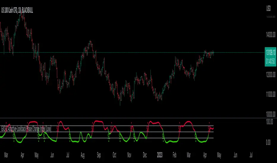
Autoback Grid Lab [trade_lexx]Autoback Grid Lab: Your personal laboratory for optimizing grid strategies.
Introduction
First of all, it is important to understand that Autoback Grid Lab is a powerful professional tool for backtesting and optimization, created specifically for traders using both grid strategies and regular take profit with stop loss.
The main purpose of this script is to save you weeks and months of manual testing and parameter selection. Instead of manually testing one combination of settings after another, Autoback Grid Lab automatically tests thousands of unique strategies on historical data, providing you with a comprehensive report on the most profitable and, more importantly, sustainable ones.
If you want to find mathematically sound, most effective settings for your grid strategy on a specific asset and timeframe, then this tool was created for you.
Key Features
My tool has functionality that transforms the process of finding the perfect strategy from a routine into an exciting exploration.
🧪 Mass testing of thousands of combinations
The script is able to systematically generate and run a huge number of unique combinations of parameters through the built-in simulator. You set the ranges, and the indicator does all the work, testing all possible options for the following grid settings:
* Number of safety orders (SO Count)
* Grid step (SO Step)
* Step Multiplier (SO Multiplier) for building nonlinear grids
* Martingale for controlling the volume of subsequent orders
* Take Profit (%)
* Stop Loss (%), with the possibility of calculating both from the entry point and from the dynamic breakeven line
* The volume of the base order (Volume BO) as a percentage of the deposit
🏆 Unique `FinalScore` rating system
Sorting strategies by net profit alone is a direct path to self—deception and choosing strategies that are "tailored" to history and will inevitably fail in real trading. To solve this problem, we have developed FinalScore, a comprehensive assessment of the sustainability and quality of the strategy.
How does it work?
FinalScore analyzes each combination not one by one, but by nine key performance metrics at once, including Net Profit, Drawdown, Profit Factor, WinRate, Sharpe coefficients, Sortino, Squid and Omega. Each of these indicators is normalized, that is, reduced to a single scale. Then, to test the strategy for strength, the system performs 30 iterations, each time assigning random weights to these 9 metrics. A strategy gets a high FinalScore only if it shows consistently high results under different evaluation criteria. This proves her reliability and reduces the likelihood that her success was an accident.
📈 Realistic backtesting engine
The test results are meaningless if they do not take into account the actual trading conditions. Our simulator simulates real trading as accurately as possible, taking into account:
* Leverage: Calculation of the required margin to open and hold positions.
* Commission: A percentage commission is charged each time an order is opened and closed.
* Slippage: The order execution price is adjusted by a set percentage to simulate real market conditions.
* Liquidation model: This is one of the most important functions. The script continuously monitors the equity of the account (capital + unrealized P&L). If equity falls below the level of the supporting margin (calculated from the current value of the position), the simulator forcibly closes the position, as it would happen on a real exchange. This eliminates unrealistic scenarios where the strategy survives after a huge drawdown.
🔌 Integration with external signals
The indicator operates in two modes:
1. `No Signal': Standard mode. The trading cycle starts immediately as soon as the previous one has been closed. Ideal for testing the "pure" mechanics of the grid.
2. `External Signal`: In this mode, a new trading cycle will start only when a signal is received from an external source. You can connect any other indicator (such as the RSI, MACD, or your own strategy) to the script and use it as a trigger to log in. This allows you to combine the power of a grid strategy with your own entry points.
📊 Interactive and informative results panel
Upon completion of the calculations, a detailed table with the TOP N best strategies appears on the screen, sorted according to your chosen criterion. For each strategy in the rating, you will see not only the key metrics (Profit, Drawdown, duration of transactions), but also all the parameters that led to this result. You can immediately take these settings and apply them in your trading.
Application Options: How To Solve Your Problems
Autoback Grid Lab is a flexible tool that can be adapted to solve various tasks, from complete grid optimization to fine—tuning existing strategies. Here are some key scenarios for its use:
1. Complete Optimization Of The Grid Strategy
This is the basic and most powerful mode of use. You can find the most efficient grid configuration for any asset from scratch.
* How to use: Set wide ranges for all key grid parameters ('SO Count`, SO Step, SO Multiplier, Martingale, TP, etc.).
* In the `No Signal` mode: You will find the most stable grid configuration that works as an independent, constantly active strategy, regardless of which-or entrance indicators.
* In the `External Signal` mode: You can connect your favorite indicator for input (for example, RSI, MACD or a complex author's script) and find the optimal grid parameters that best complement your input signals. This allows you to turn a simple signaling strategy into a full-fledged grid system.
2. Selecting the Optimal Take Profit and Stop Loss for Your Strategy
Do you already have an entry strategy, but you are not sure where it is best to put Take Profit and Stop Loss? Autoback Grid Lab can solve this problem as well.
* How to use:
1. Disable optimization of all grid parameters (uncheck SO Count, SO Step, Martingale, etc.). Set the Min value for SO Count to 0.
2. Set the ranges for iteration only for 'Take Profit` and `Stop Loss'.
3. Turn on the External Signal mode and connect your indicator with input signals.
* Result: The script will run your historical entry signals with hundreds of different TP and SL combinations and show you which stop order levels bring maximum profit with minimal risk specifically for your entry points.
3. Building a Secure Network with Risk Management
Many traders are afraid of grid strategies because of the risk of large drawdowns. With the help of the optimizer, you can purposefully find the parameters for such a grid, which includes mandatory risk management through Stop Loss.
* How to use: Enable and set the range for Stop Loss, along with other grid parameters. Don't forget to test both types of SL calculations (`From entry point` and `From breakeven line`) to determine which one works more efficiently.
* Result: You will find balanced strategies in which the grid parameters (number of orders, martingale) and the Stop Loss level are selected in such a way as to maximize profits without going beyond the acceptable risk level for you.
How To Use The Indicator (Step-By-Step Guide)
Working with the Autoback Grid Lab is a sequential process consisting of four main steps: from initial setup to analysis of the finished results. Follow this guide to get the most out of the tool.
Step 1: Initial Setup
1. Add the indicator to the chart of your chosen asset and timeframe.
2. Open the script settings. The first thing you should pay attention to is the ⚙️ Optimization Settings ⚙️ group.
3. Set the `Bars Count'. This parameter determines how much historical data will be used for testing.
* Important: The more bars you specify, the more statistically reliable the backtest results will be. We recommend using the maximum available value (25,000) to test strategies at different market phases.
* Consider: The indicator performs all calculations on the last historical bar. After applying the TradingView settings, it will take some time to load all the specified bars. The results table will appear only after the data is fully loaded. Don't worry if it doesn't appear instantly. And if an error occurs, simply switch the number of combinations to 990 and back to 1000 until the table appears.
Step 2: Optimization Configuration
At this stage, you define the "universe" of parameters that our algorithm will explore.
1. Set the search ranges (🛠 Optimization Parameters 🛠 group).
For each grid parameter that you want to optimize (for example, SO Count or `Take Profit'), you must specify three values:
* Min: The minimum value of the range.
* Max: The maximum value of the range.
* Step: The step with which the values from Min to Max will be traversed.
*Example:* If you set Min=5, Max=10, and Step=1 for SO Count, the script will test strategies with 5, 6, 7, 8, 9, and 10 safety orders.
* Tip for users: To get the first results quickly, start with a larger step (for example, TP from 0.5% to 2.5% in 0.5 increments instead of 0.1). After you identify the most promising areas, you can perform a deeper analysis by expanding the ranges around these values.
2. Set Up Money Management (Group `💰 Money Management Settings 💰`).
Fill in these fields with the values that best match your actual trading conditions. This is critically important for obtaining reliable results.
* Capital: Your initial deposit.
* Leverage: Leverage.
* Commission (%): Your trading commission as a percentage.
* Slippage (%): Expected slippage.
* Liquidation Level (%): The level of the supporting margin (MMR in %). For example, for Binance Futures, this value is usually between 0.4% and 2.5%, depending on the asset and position size. Specify this value for your exchange.
3. Select the Sorting Criterion and the Direction (Group `⚙️ Optimization Settings ⚙️').
* `Sort by': Specify the main criteria by which the best strategies will be selected and sorted. I strongly recommend using finalScore to find the most balanced and sustainable strategies.
* `Direction': Choose which trades to test: Long, Short or Both.
Step 3: Start Testing and Work with "Parts"
The total number of unique combinations generated based on your ranges can reach tens of millions. TradingView has technical limitations on the number of calculations that the script can perform at a time. To get around this, I implemented a "Parts" system.
1. What are `Part` and `Combinations in Part'?
* `Combinations in Part': This is the number of backtests that the script performs in one run (1000 by default).
* `Part`: This is the number of the "portion" of combinations that you want to test.
2. How does it work in practice?
* After you have everything set up, leave Part:1 and wait for the results table to appear. You will see the TOP N best strategies from the first thousand tested.
* Analyze them. Then, to check the next thousand combinations, just change the Part to 2 in the settings and click OK. The script will run a test for the next batch.
* Repeat this process by increasing the Part number (`3`, 4, 5...), until you reach the last available part.
* Where can I see the total number of parts? In the information row below the results table, you will find Total parts. This will help you figure out how many more tests are left to run.
Step 4: Analyze the Results in the Table
The results table is your main decision—making tool. It displays the best strategies found, sorted by the criteria you have chosen.
1. Study the performance metrics:
* Rating: Position in the rating.
* Profit %: Net profit as a percentage of the initial capital.
* Drawdown%: The maximum drawdown of the deposit for the entire test period.
* Max Length: The maximum duration of one transaction in days, hours and minutes.
* Trades: The total number of completed trades.
2. Examine the winning parameters:
* To the right of the performance metrics are columns showing the exact settings that led to this result ('SO Count`, SO Step, TP (%), etc.).
3. How to choose the best strategy?
* Don't chase after the maximum profit! The strategy with the highest profit often has the highest drawdown, which makes it extremely risky.
* Seek a balance. The ideal strategy is a compromise between high profitability, low drawdown (Drawdown) and the maximum length of trades acceptable to you (Max Length).
* finalScore was created to find this balance. Trust him — he often highlights not the most profitable, but the most stable and reliable options.
Detailed Description Of The Settings
This section serves as a complete reference for each parameter available in the script settings. The parameters are grouped in the same way as in the indicator interface for your convenience.
Group: ⚙️ Optimization Settings ⚙️
The main parameters governing the testing process are collected here.
* `Enable Optimizer': The main switch. Activates or deactivates all backtesting functionality.
* `Direction': Determines which way trades will be opened during the simulation.
* Long: Shopping only.
* Short: Sales only.
* Both: Testing in both directions. Important: This mode only works in conjunction with an External Signal, as the script needs an external signal to determine the direction for each specific transaction.
* `Signal Mode`: Controls the conditions for starting a new trading cycle (opening a base order).
* No Signal: A new cycle starts immediately after the previous one is completed. This mode is used to test "pure" grid mechanics without reference to market conditions.
* External Signal: A new cycle begins only when a signal is received from an external indicator connected via the Signal field.
* `Signal': A field for connecting an external signal source (works only in the `External Signal` mode). You can select any other indicator on the chart.
* For Long** trades, the signal is considered received if the value of the external indicator ** is greater than 0.
* For Short** trades, the signal is considered received if the value of the external indicator ** is less than 0.
* `Bars Count': Sets the depth of the history in the bars for the backtest. The maximum value (25000) provides the most reliable results.
* `Sort by`: A key criterion for selecting and ranking the best strategies in the final table.
* FinalScore: Recommended mode. A comprehensive assessment that takes into account 9 metrics to find the most balanced and sustainable strategies.
* Profit: Sort by net profit.
* Drawdown: Sort by minimum drawdown.
* Max Length: Sort by the minimum length of the longest transaction.
* `Combinations Count': Indicates how many of the best strategies (from 1 to 50) will be displayed in the results table.
* `Close last trade`: If this option is enabled, any active trade will be forcibly closed at the closing price of the last historical bar. For grid strategies, it is recommended to always enable this option in order to get the correct calculation of the final profit and eliminate grid strategies that have been stuck for a long time.
Group: 💰 Money Management Settings 💰
The parameters in this group determine the financial conditions of the simulation. Specify values that are as close as possible to your actual values in order to get reliable results.
* `Capital': The initial deposit amount for the simulation.
* `Leverage`: The leverage used to calculate the margin.
* `Slippage` (%): Simulates the difference between the expected and actual order execution price. The specified percentage will be applied to each transaction.
* `Commission` (%): The trading commission of your exchange as a percentage. It is charged at the execution of each order (both at opening and closing).
* `Liquidation Level' (%): Maintenance Margin Ratio. This is a critical parameter for a realistic test. Liquidation in the simulator occurs if the Equity of the account (Capital + Unrealized P&L) falls below the level of the supporting margin.
Group: 🛠 Optimization Parameters 🛠
This is the "heart" of the optimizer, where you set ranges for iterating through the grid parameters.
* `Part`: The portion number of the combinations to be tested. Start with 1, and then increment (`2`, 3, ...) sequentially to check all generated strategies.
* `Combinations in Part': The number of backtests performed at a time (in one "Part"). Increasing the value may speed up the process, but it may cause the script to error due to platform limitations. If an error occurs, it is recommended to switch to the step below and back.
Three fields are available for each of the following parameters (`SO Count`, SO Step, SO Multiplier, etc.):
* `Min`: Minimum value for testing.
* `Max': The maximum value for testing.
* `Step`: The step with which the values in the range from Min to Max will be iterated over.
There is also a checkbox for each parameter. If it is enabled, the parameter will be optimized in the specified range. If disabled, only one value specified in the Min field will be used for all tests.
* 'Stop Loss': In addition to the standard settings Min, Max, Step, it has an additional parameter:
* `Type`: Defines how the stop loss price is calculated.
* From entry point: The SL level is calculated once from the entry price (base order price).
* From breakeven line: The SL level is dynamically recalculated from the average position price after each new safety order is executed.
Group: ⚡️Filters⚡️
Filters allow you to filter out those results from the final table that do not meet your minimum requirements.
For each filter (`Max Profit`, Min Drawdown, `Min Trade Length`), you can:
1. Turn it on or off using the checkbox.
2. Select the comparison condition: Greater (More) or Less (Less).
3. Set a threshold value.
*Example:* If you set Less and 20 for the Min Drawdown filter, only those strategies with a maximum drawdown of less than 20% will be included in the final table.
Group: 🎨 Visual Settings 🎨
Here you can customize the appearance of the results table.
* `Position': Selects the position of the table on the screen (for example, Bottom Left — bottom left).
* `Font Size': The size of the text in the table.
* `Header Background / Data Background`: Background colors for the header and data cells.
* `Header Font Color / Data Font Color`: Text colors for the header and data cells.
Important Notes and Limitations
So that you can use the Autoback Grid Lab as efficiently and consciously as possible, please familiarize yourself with the following key features of its work.
1. It is a Tool for Analysis, not for Signals
It is extremely important to understand that this script does not generate trading signals in real time. Its sole purpose is to conduct in—depth research (**backtesting**) on historical data.
* The results you see in the table are a report on how a particular strategy would have worked in the past.
* The script does not provide alerts and does not draw entry/exit points on the chart for the current market situation.
* Your task is to take the best sets of parameters found during optimization and use them in your real trading, for example, when setting up a trading bot or in a manual trading system.
2. Features Of Calculations (This is not a "Repainting")
You will notice that the results table appears and is updated only once — when all historical bars on the chart are loaded. It does not change in real time with each tick of the price.
This is correct and intentional behavior.:
* To test thousands, and sometimes millions of combinations, the script needs to perform a huge amount of calculations. In the Pine Script™ environment, it is technically possible to do this only once, at the very last bar in history.
* The script does not show false historical signals, which then disappear or change. It provides a static report on the results of the simulation, which remains unchanged for a specific historical period.
3. Past Results do not Guarantee Future Results.
This is the golden rule of trading, and it fully applies to the results of backtesting. Successful strategy performance in the past is not a guarantee that it will be as profitable in the future. Market conditions, volatility and trends are constantly changing.
My tool, especially when sorting by finalScore, is aimed at finding statistically stable and reliable strategies to increase the likelihood of their success in the future. However, it is a tool for managing probabilities, not a crystal ball for predicting the future. Always use proper risk management.
4. Dependence on the Quality and Depth of the Story
The reliability of the results directly depends on the quantity and quality of the historical data on which the test was conducted.
* Always strive to use the maximum number of bars available (`Bars Count: 25,000`) so that your strategy is tested on different market cycles (rise, fall, flat).
* The results obtained on data for one month may differ dramatically from the results obtained on data for two years. The longer the testing period, the higher the confidence in the parameters found.
Conclusion
The Autoback Grid Lab is your personal research laboratory, designed to replace intuitive guesses and endless manual selection of settings with a systematic, data—driven approach. Experiment with different assets, timeframes, and settings ranges to find the unique combinations that best suit your trading style.

Quantify [Entry Model] | FractalystWhat’s the indicator’s purpose and functionality?
Quantify is a machine learning entry model designed to help traders identify high-probability setups to refine their strategies.
➙ Simply pick your bias, select your entry timeframes, and let Quantify handle the rest for you.
Can the indicator be applied to any market approach/trading strategy?
Absolutely, all trading strategies share one fundamental element: Directional Bias
Once you’ve determined the market bias using your own personal approach, whether it’s through technical analysis or fundamental analysis, select the trend direction in the Quantify user inputs.
The algorithm will then adjust its calculations to provide optimal entry levels aligned with your chosen bias. This involves analyzing historical patterns to identify setups with the highest potential expected values, ensuring your setups are aligned with the selected direction.
Can the indicator be used for different timeframes or trading styles?
Yes, regardless of the timeframe you’d like to take your entries, the indicator adapts to your trading style.
Whether you’re a swing trader, scalper, or even a position trader, the algorithm dynamically evaluates market conditions across your chosen timeframe.
How can this indicator help me to refine my trading strategy?
1. Focus on Positive Expected Value
• The indicator evaluates every setup to ensure it has a positive expected value, helping you focus only on trades that statistically favor long-term profitability.
2. Adapt to Market Conditions
• By analyzing real-time market behavior and historical patterns, the algorithm adjusts its calculations to match current conditions, keeping your strategy relevant and adaptable.
3. Eliminate Emotional Bias
• With clear probabilities, expected values, and data-driven insights, the indicator removes guesswork and helps you avoid emotional decisions that can damage your edge.
4. Optimize Entry Levels
• The indicator identifies optimal entry levels based on your selected bias and timeframes, improving robustness in your trades.
5. Enhance Risk Management
• Using tools like the Kelly Criterion, the indicator suggests optimal position sizes and risk levels, ensuring that your strategy maintains consistency and discipline.
6. Avoid Overtrading
• By highlighting only high-potential setups, the indicator keeps you focused on quality over quantity, helping you refine your strategy and avoid unnecessary losses.
How can I get started to use the indicator for my entries?
1. Set Your Market Bias
• Determine whether the market trend is Bullish or Bearish using your own approach.
• Select the corresponding bias in the indicator’s user inputs to align it with your analysis.
2. Choose Your Entry Timeframes
• Specify the timeframes you want to focus on for trade entries.
• The indicator will dynamically analyze these timeframes to provide optimal setups.
3. Let the Algorithm Analyze
• Quantify evaluates historical data and real-time price action to calculate probabilities and expected values.
• It highlights setups with the highest potential based on your selected bias and timeframes.
4. Refine Your Entries
• Use the insights provided—entry levels, probabilities, and risk calculations—to align your trades with a math-driven edge.
• Avoid overtrading by focusing only on setups with positive expected value.
5. Adapt to Market Conditions
• The indicator continuously adapts to real-time market behavior, ensuring its recommendations stay relevant and precise as conditions change.
How does the indicator calculate the current range?
The indicator calculates the current range by analyzing swing points from the very first bar on your charts to the latest available bar it identifies external liquidity levels, also known as BSLQ (buy-side liquidity levels) and SSLQ (sell-side liquidity levels).
What's the purpose of these levels? What are the underlying calculations?
1. Understanding Swing highs and Swing Lows
Swing High: A Swing High is formed when there is a high with 2 lower highs to the left and right.
Swing Low: A Swing Low is formed when there is a low with 2 higher lows to the left and right.
2. Understanding the purpose and the underlying calculations behind Buyside, Sellside and Pivot levels.
3. Identifying Discount and Premium Zones.
4. Importance of Risk-Reward in Premium and Discount Ranges
How does the script calculate probabilities?
The script calculates the probability of each liquidity level individually. Here's the breakdown:
1. Upon the formation of a new range, the script waits for the price to reach and tap into pivot level level. Status: "■" - Inactive
2. Once pivot level is tapped into, the pivot status becomes activated and it waits for either liquidity side to be hit. Status: "▶" - Active
3. If the buyside liquidity is hit, the script adds to the count of successful buyside liquidity occurrences. Similarly, if the sellside is tapped, it records successful sellside liquidity occurrences.
4. Finally, the number of successful occurrences for each side is divided by the overall count individually to calculate the range probabilities.
Note: The calculations are performed independently for each directional range. A range is considered bearish if the previous breakout was through a sellside liquidity. Conversely, a range is considered bullish if the most recent breakout was through a buyside liquidity.
What does the multi-timeframe functionality offer?
You can incorporate up to 4 higher timeframe probabilities directly into the table.
This feature allows you to analyze the probabilities of buyside and sellside liquidity across multiple timeframes, without the need to manually switch between them.
By viewing these higher timeframe probabilities in one place, traders can spot larger market trends and refine their entries and exits with a better understanding of the overall market context.
What are the multi-timeframe underlying calculations?
The script uses the same calculations (mentioned above) and uses security function to request the data such as price levels, bar time, probabilities and booleans from the user-input timeframe.
How does the Indicator Identifies Positive Expected Values?
Quantify instantly calculates whether a trade setup has the potential to generate positive expected value (EV).
To determine a positive EV setup, the indicator uses the formula:
EV = ( P(Win) × R(Win) ) − ( P(Loss) × R(Loss))
where:
- P(Win) is the probability of a winning trade.
- R(Win) is the reward or return for a winning trade, determined by the current risk-to-reward ratio (RR).
- P(Loss) is the probability of a losing trade.
- R(Loss) is the loss incurred per losing trade, typically assumed to be -1.
By calculating these values based on historical data and the current trading setup, the indicator helps you understand whether your trade has a positive expected value.
How can I know that the setup I'm going to trade with has a positive EV?
If the indicator detects that the adjusted pivot and buy/sell side probabilities have generated positive expected value (EV) in historical data, the risk-to-reward (RR) label within the range box will be colored blue and red .
If the setup does not produce positive EV, the RR label will appear gray.
This indicates that even the risk-to-reward ratio is greater than 1:1, the setup is not likely to yield a positive EV because, according to historical data, the number of losses outweighs the number of wins relative to the RR gain per winning trade.
What is the confidence level in the indicator, and how is it determined?
The confidence level in the indicator reflects the reliability of the probabilities calculated based on historical data. It is determined by the sample size of the probabilities used in the calculations. A larger sample size generally increases the confidence level, indicating that the probabilities are more reliable and consistent with past performance.
How does the confidence level affect the risk-to-reward (RR) label?
The confidence level (★) is visually represented alongside the probability label. A higher confidence level indicates that the probabilities used to determine the RR label are based on a larger and more reliable sample size.
How can traders use the confidence level to make better trading decisions?
Traders can use the confidence level to gauge the reliability of the probabilities and expected value (EV) calculations provided by the indicator. A confidence level above 95% is considered statistically significant and indicates that the historical data supporting the probabilities is robust. This high confidence level suggests that the probabilities are reliable and that the indicator’s recommendations are more likely to be accurate.
In data science and statistics, a confidence level above 95% generally means that there is less than a 5% chance that the observed results are due to random variation. This threshold is widely accepted in research and industry as a marker of statistical significance. Studies such as those published in the Journal of Statistical Software and the American Statistical Association support this threshold, emphasizing that a confidence level above 95% provides a strong assurance of data reliability and validity.
Conversely, a confidence level below 95% indicates that the sample size may be insufficient and that the data might be less reliable. In such cases, traders should approach the indicator’s recommendations with caution and consider additional factors or further analysis before making trading decisions.
How does the sample size affect the confidence level, and how does it relate to my TradingView plan?
The sample size for calculating the confidence level is directly influenced by the amount of historical data available on your charts. A larger sample size typically leads to more reliable probabilities and higher confidence levels.
Here’s how the TradingView plans affect your data access:
Essential Plan
The Essential Plan provides basic data access with a limited amount of historical data. This can lead to smaller sample sizes and lower confidence levels, which may weaken the robustness of your probability calculations. Suitable for casual traders who do not require extensive historical analysis.
Plus Plan
The Plus Plan offers more historical data than the Essential Plan, allowing for larger sample sizes and more accurate confidence levels. This enhancement improves the reliability of indicator calculations. This plan is ideal for more active traders looking to refine their strategies with better data.
Premium Plan
The Premium Plan grants access to extensive historical data, enabling the largest sample sizes and the highest confidence levels. This plan provides the most reliable data for accurate calculations, with up to 20,000 historical bars available for analysis. It is designed for serious traders who need comprehensive data for in-depth market analysis.
PRO+ Plans
The PRO+ Plans offer the most extensive historical data, allowing for the largest sample sizes and the highest confidence levels. These plans are tailored for professional traders who require advanced features and significant historical data to support their trading strategies effectively.
For many traders, the Premium Plan offers a good balance of affordability and sufficient sample size for accurate confidence levels.
What is the HTF probability table and how does it work?
The HTF (Higher Time Frame) probability table is a feature that allows you to view buy and sellside probabilities and their status from timeframes higher than your current chart timeframe.
Here’s how it works:
Data Request: The table requests and retrieves data from user-defined higher timeframes (HTFs) that you select.
Probability Display: It displays the buy and sellside probabilities for each of these HTFs, providing insights into the likelihood of price movements based on higher timeframe data.
Detailed Tooltips: The table includes detailed tooltips for each timeframe, offering additional context and explanations to help you understand the data better.
What do the different colors in the HTF probability table indicate?
The colors in the HTF probability table provide visual cues about the expected value (EV) of trading setups based on higher timeframe probabilities:
Blue: Suggests that entering a long position from the HTF user-defined pivot point, targeting buyside liquidity, is likely to result in a positive expected value (EV) based on historical data and sample size.
Red: Indicates that entering a short position from the HTF user-defined pivot point, targeting sellside liquidity, is likely to result in a positive expected value (EV) based on historical data and sample size.
Gray: Shows that neither long nor short trades from the HTF user-defined pivot point are expected to generate positive EV, suggesting that trading these setups may not be favorable.
What machine learning techniques are used in Quantify?
Quantify offers two main machine learning approaches:
1. Adaptive Learning (Fixed Sample Size): The algorithm learns from the entire dataset without resampling, maintaining a stable model that adapts to the latest market conditions.
2. Bootstrap Resampling: This method creates multiple subsets of the historical data, allowing the model to train on varying sample sizes. This technique enhances the robustness of predictions by ensuring that the model is not overfitting to a single dataset.
How does machine learning affect the expected value calculations in Quantify?
Machine learning plays a key role in improving the accuracy of expected value (EV) calculations. By analyzing historical price action, liquidity hits, and market bias patterns, the model continuously adjusts its understanding of risk and reward, allowing the expected value to reflect the most likely market movements. This results in more precise EV predictions, helping traders focus on setups that maximize profitability.
What is the Kelly Criterion, and how does it work in Quantify?
The Kelly Criterion is a mathematical formula used to determine the optimal position size for each trade, maximizing long-term growth while minimizing the risk of large drawdowns. It calculates the percentage of your portfolio to risk on a trade based on the probability of winning and the expected payoff.
Quantify integrates this with user-defined inputs to dynamically calculate the most effective position size in percentage, aligning with the trader’s risk tolerance and desired exposure.
How does Quantify use the Kelly Criterion in practice?
Quantify uses the Kelly Criterion to optimize position sizing based on the following factors:
1. Confidence Level: The model assesses the confidence level in the trade setup based on historical data and sample size. A higher confidence level increases the suggested position size because the trade has a higher probability of success.
2. Max Allowed Drawdown (User-Defined): Traders can set their preferred maximum allowed drawdown, which dictates how much loss is acceptable before reducing position size or stopping trading. Quantify uses this input to ensure that risk exposure aligns with the trader’s risk tolerance.
3. Probabilities: Quantify calculates the probabilities of success for each trade setup. The higher the probability of a successful trade (based on historical price action and liquidity levels), the larger the position size suggested by the Kelly Criterion.
What is a trailing stoploss, and how does it work in Quantify?
A trailing stoploss is a dynamic risk management tool that moves with the price as the market trend continues in the trader’s favor. Unlike a fixed take profit, which stays at a set level, the trailing stoploss automatically adjusts itself as the market moves, locking in profits as the price advances.
In Quantify, the trailing stoploss is enhanced by incorporating market structure liquidity levels (explain above). This ensures that the stoploss adjusts intelligently based on key price levels, allowing the trader to stay in the trade as long as the trend remains intact, while also protecting profits if the market reverses.
Why would a trader prefer a trailing stoploss based on liquidity levels instead of a fixed take-profit level?
Traders who use trailing stoplosses based on liquidity levels prefer this method because:
1. Market-Driven Flexibility: The stoploss follows the market structure rather than being static at a pre-defined level. This means the stoploss is less likely to be hit by small market fluctuations or false reversals. The stoploss remains adaptive, moving as the market moves.
2. Riding the Trend: Traders can capture more profit during a sustained trend because the trailing stop will adjust only when the trend starts to reverse significantly, based on key liquidity levels. This allows them to hold positions longer without prematurely locking in profits.
3. Avoiding Premature Exits: Fixed stoploss levels may exit a trade too early in volatile markets, while liquidity-based trailing stoploss levels respect the natural flow of price action, preventing the trader from exiting too soon during pullbacks or minor retracements.
🎲 Becoming the House: Gaining an Edge Over the Market
In American roulette, the casino has a 5.26% edge due to the presence of the 0 and 00 pockets. On even-money bets, players face a 47.37% chance of winning, while true 50/50 odds would require a 50% chance. This edge—the gap between the payout odds and the true probabilities—ensures that, statistically, the casino will always win over time, even if individual players win occasionally.
From a Trader’s Perspective
In trading, your edge comes from identifying and executing setups with a positive expected value (EV). For example:
• If you identify a setup with a 55.48% chance of winning and a 1:1 risk-to-reward (RR) ratio, your trade has a statistical advantage over a neutral (50/50) probability.
This edge works in your favor when applied consistently across a series of trades, just as the casino’s edge ensures profitability across thousands of spins.
🎰 Applying the Concept to Trading
Like casinos leverage their mathematical edge in games of chance, you can achieve long-term success in trading by focusing on setups with positive EV and managing your trades systematically. Here’s how:
1. Probability Advantage: Prioritize trades where the probability of success (win rate) exceeds the breakeven rate for your chosen risk-to-reward ratio.
• Example: With a 1:1 RR, you need a win rate above 50% to achieve positive EV.
2. Risk-to-Reward Ratio (RR): Even with a win rate below 50%, you can gain an edge by increasing your RR (e.g., a 40% win rate with a 2:1 RR still has positive EV).
3. Consistency and Discipline: Just as casinos profit by sticking to their mathematical advantage over thousands of spins, traders must rely on their edge across many trades, avoiding emotional decisions or overleveraging.
By targeting favorable probabilities and managing trades effectively, you “become the house” in your trading. This approach allows you to leverage statistical advantages to enhance your overall performance and achieve sustainable profitability.
What Makes the Quantify Indicator Original?
1. Data-Driven Edge
Unlike traditional indicators that rely on static formulas, Quantify leverages probability-based analysis and machine learning. It calculates expected value (EV) and confidence levels to help traders identify setups with a true statistical edge.
2. Integration of Market Structure
Quantify uses market structure liquidity levels to dynamically adapt. It identifies key zones like swing highs/lows and liquidity traps, enabling users to align entries and exits with where the market is most likely to react. This bridges the gap between price action analysis and quantitative trading.
3. Sophisticated Risk Management
The Kelly Criterion implementation is unique. Quantify allows traders to input their maximum allowed drawdown, dynamically adjusting risk exposure to maintain optimal position sizing. This ensures risk is scientifically controlled while maximizing potential growth.
4. Multi-Timeframe and Liquidity-Based Trailing Stops
The indicator doesn’t just suggest fixed profit-taking levels. It offers market structure-based trailing stop-loss functionality, letting traders ride trends as long as liquidity and probabilities favor the position, which is rare in most tools.
5. Customizable Bias and Adaptive Learning
• Directional Bias: Traders can set a bullish or bearish bias, and the indicator recalculates probabilities to align with the trader’s market outlook.
• Adaptive Learning: The machine learning model adapts to changes in data (via resampling or bootstrap methods), ensuring that predictions stay relevant in evolving markets.
6. Positive EV Focus
The focus on positive EV setups differentiates it from reactive indicators. It shifts trading from chasing signals to acting on setups that statistically favor profitability, akin to how professional quant funds operate.
7. User Empowerment
Through features like customizable timeframes, real-time probability updates, and visualization tools, Quantify empowers users to make data-informed decisions.
Terms and Conditions | Disclaimer
Our charting tools are provided for informational and educational purposes only and should not be construed as financial, investment, or trading advice. They are not intended to forecast market movements or offer specific recommendations. Users should understand that past performance does not guarantee future results and should not base financial decisions solely on historical data.
Built-in components, features, and functionalities of our charting tools are the intellectual property of @Fractalyst use, reproduction, or distribution of these proprietary elements is prohibited.
By continuing to use our charting tools, the user acknowledges and accepts the Terms and Conditions outlined in this legal disclaimer and agrees to respect our intellectual property rights and comply with all applicable laws and regulations.